This post is the next part of our previous post Financial Calculations in MATLAB named as Implementation of Black Litterman Approach in MATLAB, so if you haven't read that then you can't understand what's going on here so, its better that you should first have a look at that post. Moreover, as this code is designed after a lot of our team effort so its not free but we have placed a very small cost of $20. So you can buy it easily by clicking on the above button.In the previous post, we have covered five steps in which we first get the financial stock data, then converted it to common currency and after that we calculated the expected returns and covariance matrix and then plot the frontiers with and without risk free rate of 3%. Now in this post, we are gonna calculate the optimal asset allocation, average return after the back test, calculation of alphas and betas of the system and finally the implementation of black-litterman approach. First five steps are explained in the previous tutorial and the next four steps for Implementation of Black Litterman Approach in MATLAB are gonna discuss in this tutorial, which are as follows:
You may also like to read:
In this part of the problem,I calculated the optimal asset allocation in the different years by choosing a constant required return. I chose the constant required return equal to 0.01 and used the highest_slope_portfolio function and plot the graphs. The code used in MATLAB is shown in the below:
ConsRet=0.010 for w=1:10 [xoptCR(:,w), muoptCR(w), sigoptCR(w)] = highest_slope_portfolio( covmat{1,w}, ConsRet , estReturn(w,:)', stdRet(w,:) ); End
The result for this part is shown in the Figure 3. For a constant required return of 0.01, portfolio turnover for each year has increased approximately by 2%.
In this part of the assignment, it was asked to perform a back test for the optimized portfolios and calculate the average return and the standard deviation for this portfolio. Average return is the average of expected return for the corresponding year and it is calculated by the below code in MATLAB, where w is varying from 1 to 10 to calculate for all the 10 years.
BTreturn(w,:)=estReturn(w,:)*xoptCR(:,w);Results obtained after the back test for the optimized portfolios for average return are shown in table3 below:
Average Return after the back test | |
1st year | 0.1158 |
2nd year | 0.0889 |
3rd year | 0.0797 |
4th year | 0.0628 |
5th year | -0.0660 |
6th year | -0.4323 |
7th year | -5.1212 |
8th year | -0.6820 |
9th year | 0.2891 |
10th year | 0.1691 |
Table : Average return after the back test
The standard deviation of the rate of return is a measure of risk. It is defined as the square root of the variance, which in turn is the expected value of the squared deviations from the expected return. The higher the volatility in outcomes, the higher will be the average value of these squared deviations. Therefore, variance and standard deviation measure the uncertainty of outcomes. Symbolically,
BTstd(w,:)=sqrt(stdRet(w,:).^2*(xoptCR(:,w).^2));The results of standard deviation for the 10 years are as follows:
Standard Deviation after the back test | |
1st year | 0.2942 |
2nd year | 0.1833 |
3rd year | 0.1799 |
4th year | 0.1733 |
5th year | 0.4026 |
6th year | 1.5834 |
7th year | 16.1279 |
8th year | 2.1722 |
9th year | 1.0430 |
10th year | 0.4949 |
FTLC= hist_stock_data('01111993','01112013','^FTLC','frequency','m'); LRFTLC=diff(log(FTLC.Close));After that I calculated the expected return of one unit of each asset based on the model which gave me the total covariance matrix for the single and multi indexed model. Finally, I calculated the alpha and beta for the model. The MATLAB code used for performing these actions is shown below:
for i = 1:7 mdl_si{i} = LinearModel.fit(LRFTLC, logRet(:,i), 'linear'); mdl_ret_s(i) = mdl_si{i}.Coefficients.Estimate(1:2)' * [1; 12*mean(LRFTLC)]; mdl_cov_s(i) = mdl_si{i}.RMSE^2; alpha_s = [mdl_si{i}.Coefficients.Estimate(1), alpha_s]; beta_s = [mdl_si{i}.Coefficients.Estimate(2), beta_s]; endAs a result, alphas and betas of the system are obtained which are shown in the table below:
Aplha | Beta |
0.0068 | 0.1748 |
0.0057 | 0.0335 |
0.0050 | 0.0528 |
0.0063 | 0.0552 |
0.0030 | 0.0249 |
0.0035 | 0.0083 |
0.0047 | 0.0289 |
Table: Alpha & beta of the model
In this part, I have finally implemented the Black Litterman approach on the data available. Black Litterman approach involves the below steps:
Few MATLAB Projects:
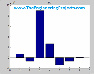
gamma = 1.9; tau = .3; for w=1:10 ind=[(w-1)*12+1 (w+10)*12]; logRet2=logRet(ind(1):ind(2),:); for i=1:7 OplogRet(:,i)=logRet2(i,:).*xoptCR(i,w)'*100; end covmatOP{1,w}=12*cov(OplogRet); end for w=1:10 Opweig(:,w)=xoptCR(:,w); Pi{w}= gamma *covmatOP{1,w}* Opweig(:,w); end figure for w=1:10 title('BL'); hold on; bar(Pi{w}) hold on; endThat's all for today, hope it will help you all in some way. If you have any questions then ask in comments and I will try my best to resolve them.
After that I calculated Expected Returns & Covariance Matrix for all these data for the last 10 years and finally plot them. Moreover, I have also plotted the frontiers with risk free rate of 3% so that the ideal and realistic conditions can be compared. So, here are the overall steps we are gonna cover in this project:
You may also like to read:
Stocks = hist_stock_data('X', 'Y', 'Z', 'frequency', 'm')
snp500 = hist_stock_data('01111993','01112013','^GSPC','frequency','m'); NDX=hist_stock_data('01111993','01112013','^NDX','frequency','m'); GSPTSE=hist_stock_data('01111993','01112013','^GSPTSE','frequency','m'); DAX = hist_stock_data('01111993','01112013','^GDAXI','frequency','m'); CAC40=hist_stock_data('01111993','01112013','^FCHI','frequency','m'); FTAS=hist_stock_data('01111993','01112013','^FTAS','frequency','m'); SSMI=hist_stock_data('01111993','01112013','^SSMI','frequency','m');
The first two values were in US dollars, while third one was in CAD dollars, fourth and fifth values were in Euros, sixth were in GBP and the last one was in Swiss France. Hence, there was a need to convert all these currencies into one currency as instructed. I converted all of them into US dollars. In order to convert them, I first defined the exchange rate between these currencies and the US dollars using the below code:
GBP2USD=1.6; EURO2USD=1.34; CAD2USD=0.95; SF2USD=1.08;After defining the exchange rate, I applied it to all the currencies using the below code:
GSPTSE=CurrencyConvert(GSPTSE, CAD2USD); DAX=CurrencyConvert(DAX, EURO2USD); CAC40=CurrencyConvert(CAC40, EURO2USD); FTAS=CurrencyConvert(FTAS, GBP2USD); SSMI=CurrencyConvert(SSMI, SF2USD);Now all the currencies for the financial stock indices for 7 sectors are obtained in US dollars.
In this part, we calculated the expected returns and covariance matrix in annual steps for a period of 10 years. I used the data for 7 markets or sectors were obtained in the first step and calculated their expected returns and covariance matrix. The expected rate of return is a probability-weighted average of the rates of return in each scenario. We may write the expected return as:
Where,First of all, I initialized a column matrix and filled it with the above data and took log of each data separately by using MATLAB commands as follows:
covmat=cell(1,11); ret=flipud([log(SSMI.Close) log(FTAS.Close) log(CAC40.Close) log(DAX.Close) log(GSPTSE.Close) log(snp500.Close) log(NDX.Close)]);
Further, I calculated the differences between adjacent elements of each data using the diff command in MATLAB.
logRet=[diff(ret(:,1)) diff(ret(:,2)) diff(ret(:,3)) diff(ret(:,4)) diff(ret(:,5)) diff(ret(:,6)) diff(ret(:,7))];
Expected return is nothing other than a guaranteed rate of return. However, it can be used to forecast the future value of a market, and it also provides a guide from which to measure actual returns. Hence to calculate the expected return, I first take two indices with w as a variable where w = 1:10 and calculated these indices for all the values of w and finally took mean value of each data with these two indices as follows:
ind=[(w-1)*12+1 (w+10)*12]; estReturn(w,:)=[mean(logRet(ind(1):ind(2),1)) mean(logRet(ind(1):ind(2),2)) mean(logRet(ind(1):ind(2),3)) mean(logRet(ind(1):ind(2),4)) mean(logRet(ind(1):ind(2),5)) mean(logRet(ind(1):ind(2),6)) mean(logRet(ind(1):ind(2),7))];
The above values calculated for all the 10 times and hence it is placed within a for loop. estReturn gives us the estimated return for a single month and now there’s a need to convert it to annual return, which is accomplished by below command, simply by mutilpying it with 12.
estReturn(w,:)=estReturn(w,:)*12;
After the calculation of expected return annually, I used the command var(X) to calculate the variance of the data. Although it was not asked to calculate in the problem but in order to calculate the covariance, it is required to first obtain the data such that each row of the matrix becomes an observation and each column is a variable. The command used for the calculation of variance is as shown below:
stdRet(w,:)=sqrt(12*var([ logRet(ind(1):ind(2),1) logRet(ind(1):ind(2),2) logRet(ind(1):ind(2),3) logRet(ind(1):ind(2),4) logRet(ind(1):ind(2),5) logRet(ind(1):ind(2),6) logRet(ind(1):ind(2),7)]));
Finally, I used the MATLAB command cov(x) to calculate the covariance of the data. The syntax used is:
Y = cov(X)Where,
Expected Return | SSMI | FTAS | CAC40 | DAX | GSPTSE | SNP50 | NDX |
1st year | 0.0625 | 0.0373 | 0.0524 | 0.0632 | 0.0700 | 0.0848 | 0.0644 |
2nd year | 0.0954 | 0.0531 | 0.0762 | 0.0846 | 0.0884 | 0.0921 | 0.1290 |
3rd year | 0.0872 | 0.0506 | 0.0972 | 0.0940 | 0.0915 | 0.0763 | 0.1004 |
4th year | 0.0742 | 0.0457 | 0.0814 | 0.0925 | 0.0747 | 0.0610 | 0.0835 |
5th year | 0.0006 | -0.0064 | 0.0122 | 0.0147 | 0.0321 | -0.0058 | 0.0110 |
6th year | -0.0112 | 0.0007 | -0.0039 | 0.0103 | 0.0537 | -0.0055 | 0.0115 |
7th year | -0.0144 | -0.0069 | -0.0356 | 0.0115 | 0.0494 | -0.0148 | -0.0307 |
8th year | -0.0314 | -0.0034 | -0.0573 | -0.0041 | 0.0295 | -0.0048 | -0.0080 |
9th year | 0.0081 | 0.0180 | -0.0209 | 0.0359 | 0.0454 | 0.0198 | 0.0470 |
10th year | 0.0431 | 0.0529 | 0.0228 | 0.0907 | 0.0644 | 0.0575 | 0.1007 |
Table 1: Expected Returns for 10 years
Covariance Matrix for 1st year | ||||||
SSMI | FTAS | CAC40 | DAX | GSPTSE | SNP50 | NDX |
0.0334 | 0.0191 | 0.0285 | 0.0324 | 0.0168 | 0.0190 | 0.0196 |
0.0191 | 0.0201 | 0.0234 | 0.0271 | 0.0155 | 0.0169 | 0.0257 |
0.0285 | 0.0234 | 0.0434 | 0.0444 | 0.0211 | 0.0226 | 0.0380 |
0.0324 | 0.0271 | 0.0444 | 0.0609 | 0.0252 | 0.0280 | 0.0527 |
0.0168 | 0.0155 | 0.0211 | 0.0252 | 0.0268 | 0.0198 | 0.0342 |
0.0190 | 0.0169 | 0.0226 | 0.0280 | 0.0198 | 0.0234 | 0.0379 |
0.0196 | 0.0257 | 0.0380 | 0.0527 | 0.0342 | 0.0379 | 0.1411 |
Covariance Matrix for 2nd year | ||||||
SSMI | FTAS | CAC40 | DAX | GSPTSE | SNP50 | NDX |
0.0318 | 0.0179 | 0.0273 | 0.0322 | 0.0162 | 0.0185 | 0.0235 |
0.0179 | 0.0180 | 0.0213 | 0.0258 | 0.0151 | 0.0161 | 0.0269 |
0.0273 | 0.0213 | 0.0404 | 0.0427 | 0.0209 | 0.0219 | 0.0390 |
0.0322 | 0.0258 | 0.0427 | 0.0590 | 0.0255 | 0.0279 | 0.0503 |
0.0162 | 0.0151 | 0.0209 | 0.0255 | 0.0265 | 0.0193 | 0.0367 |
0.0185 | 0.0161 | 0.0219 | 0.0279 | 0.0193 | 0.0230 | 0.0394 |
0.0235 | 0.0269 | 0.0390 | 0.0503 | 0.0367 | 0.0394 | 0.1014 |
Covariance Matrix for 3rd year | ||||||
SSMI | FTAS | CAC40 | DAX | GSPTSE | SNP50 | NDX |
0.0314 | 0.0181 | 0.0280 | 0.0320 | 0.0164 | 0.0186 | 0.0237 |
0.0181 | 0.0181 | 0.0214 | 0.0261 | 0.0152 | 0.0160 | 0.0270 |
0.0280 | 0.0214 | 0.0397 | 0.0433 | 0.0212 | 0.0224 | 0.0399 |
0.0320 | 0.0261 | 0.0433 | 0.0579 | 0.0259 | 0.0282 | 0.0509 |
0.0164 | 0.0152 | 0.0212 | 0.0259 | 0.0266 | 0.0194 | 0.0371 |
0.0186 | 0.0160 | 0.0224 | 0.0282 | 0.0194 | 0.0227 | 0.0395 |
0.0237 | 0.0270 | 0.0399 | 0.0509 | 0.0371 | 0.0395 | 0.1014 |
In this part, it was asked to plot the 11 different frontiers in one figure. The concept of efficient frontier was introduced by Harry Markowitz and it is defined as if a portfolio or a combination of assets has the best expected rate of return for the level of risk, it is facing, then it will be referred as “efficient”.
Few more MATLAB Projects:
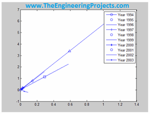
In order plot them, I used the below code in MATLAB, I used different markers for different plots so that they could be distinguished from one another quite easily. Moreover, I used the command legend in order to show the respective years for which the graphs are plotted. RF is a variable which indicate the risk-free rate and as it is asked to operate under efficient frontier that’s why risk-free rate is equal to zero.
RF=0; for w=1:10 [xopt(:,w), muopt(w), sigopt(w)] = highest_slope_portfolio( covmat{1,w}, RF, estReturn(w,:)', stdRet(w,:) ); end mker=['o' '+' '*' '.' 'x' 's' 'd' '^' '>' '<'] figure for w=1:10 plot (sigopt(w), muopt(w) ,'Marker', mker(w)); hold on; plot (0, RF, 'o'); hold on; RF_p1 = [0 sigopt(w) 2* sigopt(w)]; opt1_p = [.02 muopt(w) (2 * muopt(w) - RF) ]; line(RF_p1, opt1_p ); end legend('Year 1994', 'Year 1995', 'Year 1996', 'Year 1997','Year 1998','Year 1999','Year 2000', 'Year 2001', 'Year 2002', 'Year 2003')In this code, first of all I used highest_slope_portfolio function. This function finds the portfolio with the highest slope. Results are shown in the below figure annually:
The plot in Part (c) was about the efficient frontier with risk rate equal to zero i.e. operating in an ideal condition while in this part, it was asked to plot the same graphs but this time include a risk-free rate of 3%. Hence I used the same code as for the previous part but only this time I used RF = 0.03 as I needed to include a risk free rate of 3%. The code used in MATLAB for this part is shown below:
RF=0.03; %the risk free rate for w=1:10 [xoptRF{w}, muoptRF(w), sigoptRF(w)] = highest_slope_portfolio( covmat{1,w}, RF, estReturn(w,:)', stdRet(w,:) ); end figure for w=1:10 plot (sigoptRF(w), muoptRF(w) ,'Marker', mker(w)); hold on; plot (0, RF, 'o'); hold on; RF_p1 = [0 sigoptRF(w) 2* sigoptRF(w)]; opt1_p = [.02 muoptRF(w) (2 * muoptRF(w) - RF) ]; line(RF_p1, opt1_p ); end legend('Year 1994', 'Year 1995', 'Year 1996', 'Year 1997','Year 1998','Year 1999','Year 2000', 'Year 2001', 'Year 2002', 'Year 2003')
The result for this part i.e. after including a risk-free rate of 3% is shown in the figure below. If the Figure 1 and Figure 2 are closely examined then one can see the clear difference. When the risk-free rate was considered zero, all the expected estimate graphs were in positive direction depicting the profit annually while after adding a risk-free rate of 3%, few of the graphs went in the negative direction depicting the loss in those years. Hence adding the risk factor may cause the business to get deceased and it may even cause it to decline continuously which results in disaster.
That's all for today, in the coming post, I will calculate more financial terms like Optimal asset allocation, average return, standard deviation and much more, so stay tuned and have fun.