So you've installed a beautiful new solar energy system around your house or property. You're saving tons on your electric bill and never have to worry about blackouts, power surges, or planned outages—you control your power source now. Here's the problem: What do you do when you need to dispose of everything?
Eventually, you will need to replace the solar panels and the solar battery, which powers the whole system. Disposing of solar batteries isn't exactly simple, and it needs to be handled with the utmost care. But it is easy to navigate if you know the proper steps to take—and what to avoid. Here's our complete guide.
Disposing of the Battery
If you've recently purchased a solar energy system or portable solar generator, you know the current ...
Hello friends, welcome back to our tutorials on PLC ladder logic programming. Today we will talk about batch process control and take one project from our factory to understand, implement, and simulate. So without any further delay, let’s jump into the tutorial by asking what is batch process is if it is different from other online processes. Well! The batch process is defined as a process that starts by operating continuously till the end of the cycle without any interaction with the users. For you guys, it’s cool to know that most of the processes you might meet in the industry of batch-type processing. Do you like me to give an example? Well! The Silo cement process is a batch process, and food and beverages manufacturing are also good examples of batch processes. So what do we have tod ...
Hi, my friends, and I hope you are doing great today! We have today one interesting topic that you have seen everywhere you go, but you might not notice it! That is what the so-called binary coded decimal (BCD) is. So what’s that? Well! When you are waiting for your turn at the front of a wicket in the bank. You see 7-segmented displays that show numbers in digits. So how do these counter displays work? The BCD is the idea behind how these displays work. Numbers can be represented in many formats. Some of these formats are readable for the public which is the decimal pr the digits 0, 1, 2, .., 9. On the other side, there is another number format which is not readable to general people. Still, it is essential for computation and computer processing like binary format and hexadecimal formats ...
Welcome to today's article on our comprehensive Raspberry Pi 4 programming guide. As we saw in the previous article, the Raspberry Pi 4 may power a single seven-segment display. In addition, we also interfaced a Raspberry Pi with 4 Seven-Segment Display Modules to display the time. However, this guide will show you how to construct a Raspberry Pi 4 crypto miner that uses very little electricity.
Cryptocurrencies have been the subject of widespread conversation for some time now. It's possible to use your computer to create them, and they can be used as currency. Because of this, the Raspberry Pi can also be used for Bitcoin mining. It's also possible to mine other cryptocurrencies. One drawback of mining is that the cost of electricity often excee ...
The world of large format 3D printing is dominated by a few key players who have emerged as the pioneers in this rapidly growing industry. Below are some of the biggest large format 3D printing companies and how they stand to benefit from this revolution:
Stratasys: Stratasys is a leading provider of large format 3D printing solutions, offering a range of industrial-grade printers that are capable of producing high-quality prototypes and end-use parts. With its powerful proprietary Fused Deposition Modeling (FDM) technology, Stratasys is well positioned to capitalize on the growing demand for large format 3D Printing solutions.
HP: HP is one of the largest and most well-known technology companies in the world, and it has recently entered the larg ...
Thank you for being here for today's tutorial of our in-depth Raspberry Pi programming tutorial. The previous tutorial taught us how to install a PIR sensor on a Raspberry Pi 4 to create a motion detector. However, this tutorial will teach you how to connect a single seven-segment display to a Raspberry Pi 4. In the following sections, we will show you how to connect a Raspberry Pi to a 4-digit Seven-Segment Display Module so that the time can be shown on it.
Seven-segment displays are a simple type of Display that use eight light-emitting diodes to show off decimal numbers. It's common to find it in gadgets like digital clocks, calculators, and electronic meters that show numbers. Raspberry Pi, built around an ARM chip, is widely acknowledged as ...
Hello friends, I hope you all are doing well. Today, I am going to share the 4th chapter of Section-III in our Raspberry Pi programming course. In the previous lecture, we studied the Interfacing of IR sensor with Raspberry Pi 4. In this guide, you'll learn how to interface a PIR sensor with Raspberry Pi to create a motion detector. A passive infrared (PIR) sensor is a straightforward yet effective tool for motion detection.
As a bonus, a piezo speaker will play an audio clip whenever motion is detected. GPIO pins are required for both of these accessories. This tutorial is a great starting point for those who have never worked with electronic components and circuits.
These sensors are used in traditional, old-generation security
systems. In con ...
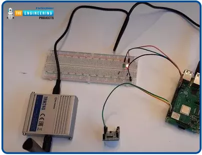
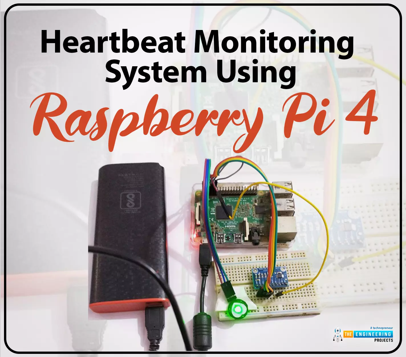
Hello friends, I hope you all are doing great. Welcome to the 11th lecture of Section-III in the Raspberry Pi 4 Programming Series. In the previous tutorial, we discussed the interfacing of the Fingerprint sensor with Raspberry Pi 4. Today, we are going to discuss another sensor named the Pulse rate sensor and will interface it with Raspberry Pi 4.The field of healthcare monitoring has long been seen as a potential use
case for IoT i.e. examining the health
instead of regular checkups and local doctors. Using sensors,
your vital signs can be monitored and transmitted in real time, allowing
a physician on the other side or even an AI to analyze the data and
provide an accurate diagnosis. That does seem somewhat futuristic.
However, we are making steady progress in that direction ...
Hi, my friends. Welcome to share a new tutorial in our ladder logic programming series. Today we will discuss counters in ladder logic programming using an expert’s view. So let’s wear the glasses of an expert in ladder logic programming and look deeply into counters, the types of counters, their variables and bits. In addition, techniques of using counters to solve a different kinds of problems that need counting. And without questions like every time, we will enjoy practicing programming and simulating all about counters. So with no further delay, let’s jump into our tutorial and nail that counters.
Counters in real life
Tell me, guys, if you can imagine an industrial project or machine that does not need to count parts, products, or processing cycles. Actually, in most cases in indust ...
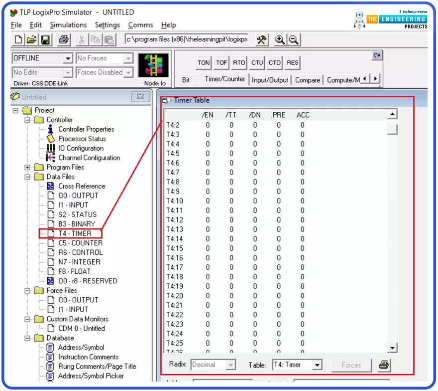
Believing in the essence of timers in ladder logic programming, we come today with a new tutorial in which we are going to show you all about timers, the types of timers, what’s inside timers’ block of parameters, variables, and bits. In addition, techniques for using timers will be explored, and for sure, we are going to practice what we learn using the simulator. So let’s get started with our tutorial.
Timers in ladder logic programming
Guys, this is not the first time we’ve talked about timers. However, this time we are going to look into timers deeply and use the glasses of practical approach. So figure 1 shows the most important types of timers in ladder logic from left to right: the on-delay, off-delay, and retentive timers. There are differences in functionality. However, they all ...