Java developers are the backbone of many successful businesses. They bring a wealth of experience and knowledge to the table, making them an invaluable asset for any company looking to stay competitive in today’s market. With Java being one of the most widely used programming languages, hiring a Java developer is often seen as the best investment for any business looking to develop their own software applications or products. From its wide industry usage to its mature ecosystem and strong community, there's no doubt that Java developers are some of the most sought-after professionals in tech today. In this article, we'll discuss why investing in a skilled Java developer may be your best bet when it comes to taking your business forward. Java competitors are C#(C Sharp), Python, PHP etc.
...
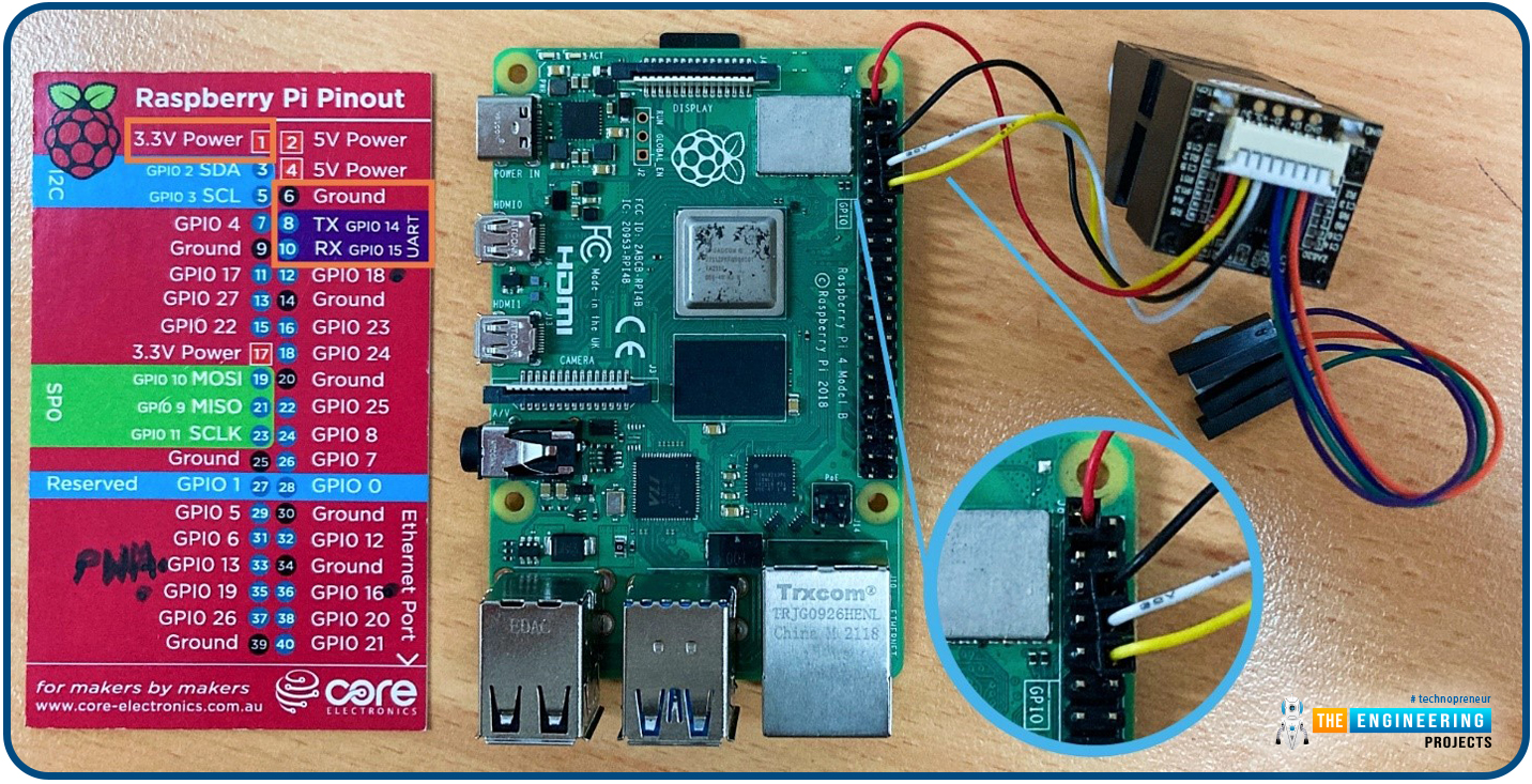
Welcome to the next tutorial of our raspberry pi 4 programming course. The last guide covered connecting a Sharp infrared distance measurement sensor to a Raspberry Pi 4. Infrared (IR) sensors were demonstrated to be widely used for nearby object recognition and motion tracking. But in this session, we'll utilize Raspberry Pi 4 to create a radio-frequency (RF) remote control that can be used to operate the gadgets wirelessly. With the help of this RF remote control, we can Power On/Off the devices.
Components
Transmitter Side
RF Transmitter
HT12E IC
4 Push Buttons
750k resistor
9 Volt battery
Receiver Side
Raspberry Pi
16x2 LCD
10K POT
Breadboard
1K Resistor (Five)
33K resistor
HT12D IC
RF Receiver
LEDs (Five)
4 10K resistor
Jumper wires
RF Module
This ...
Hello friends, I hope all are fine. Today, we are going to share the 3rd chapter of Section-III in our Raspberry Pi Programming Course. In our previous lecture, we interfaced the Soil Moisture Sensor with Raspberry Pi 4. Today, we are going to Interface the Infrared(IR) sensor with RPi4. IR Sensor is typically employed for the presence/motion detection of objects in the immediate area. With their low power consumption, straightforward design, and user-friendly features, IR sensors are a popular choice for detection purposes. Infrared(IR) impulses are invisible to the naked eye and lie between the visible and microwave parts of the electromagnetic spectrum. So let's get started:
Components Required
To learn how an IR sensor detects the existence o ...
Thank you for joining us today for our in-depth Raspberry Pi programming tutorial. The previous guide covered the steps necessary to connect a fingerprint scanner to a Raspberry Pi 4. In addition, we developed a python script to complement the sensor's ability to identify fingerprints. Yet, in this guide, we'll discover how to interface a ws2812 RGB to a Raspberry Pi 4.
Bright, colorful lights are the best, and this tutorial shows you how to set up Fully Configurable WS2812B led strips to run on a Pi 4 computer as quickly and flexibly as possible. In that manner, you can have the ambiance of your home reflect your tastes.
In most cases, when people talk about a "WS2812B Strip," they mean a long piece of extensible PCB with a bunch of different RG ...
Hello friends, I hope you all are going great. Today, I am going to share the 10th tutorial of Section-III in our Raspberry Pi Programming Course. In our previous tutorial, we interfaced a Gas Sensor MQ-2 with Raspberry Pi 4. Today, we will be interfacing a Fingerprint Sensor with Raspberry Pi today.
After appearing only in science fiction films until recently, fingerprint sensors are often employed to confirm an individual's identity in various contexts. Today, fingerprint-based systems are used for everything from checking in at the office to verifying an employee's identity at the bank, withdrawing cash from an ATM, and proving one's identity at a government agency. For identifying purposes, fingerprint-detecting technology has been used for so ...
We all know technology is not only changing trends and habits, but it is also reshaping the way we live our daily lives. We are not talking about centuries ago, but even if we examine the previous two decades, everything, from our communication style to our travel means, from our shopping habits to our entertainment industry, is changing rapidly, and this has both pros and cons. In a broader view, we can say that positive impacts are more dominant than negative effects on our lives. Maybe you have the opposite opinion, but I can prove this with the help of a simple and general example that I am going to discuss in detail with you. Just like almost every other sport and game, poker has some visible technical changes, and people can play poker online. Clients and casinos are getting more and ...
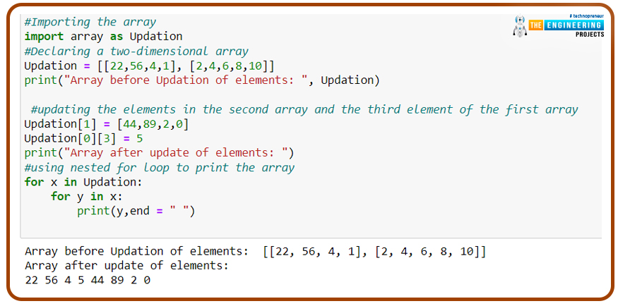
Hello learners! Welcome to the next episode of the arrays, in which we are moving towards the details of the arrays at an advanced level. In the previous lecture, we covered the introductions and fundamentals of arrays, dimensional arrays, and array operations. One must know that the working of the arrays does not end with simple operations, and there is a lot to learn about them. Arrays and their types are important topics in programming, and if we talk about Python, the working and concepts of the array in Python are relatively simple and more effective. The details of the advanced types of arrays will prove this statement. We have a lot of data to share with you, and for this reason, we have arranged this lecture. It is important to understand the reasons behind the reading of this lect ...
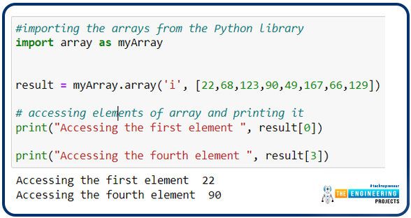
Hello Python programmers! Welcome to the engineering projects where you will find the best learning data in a precise way. We are dealing with Python nowadays, and today, the topic of discussion is the arrays in the language. We have seen different data types in Python and discussed a lot about them in detail till now. In the previous lecture, we saw the details of the procedures in dictionaries. There are certain ways to store the data in the different types of sequences, and we have highlighted a lot about almost all of them. It is time to discuss the arrays, but before this, it is better to understand the objectives of this lecture:
Introduction to arrays
Difference between contiguous and non-contiguous memory locations
One-dimensional arrays
Functions in arrays
What are Arra ...
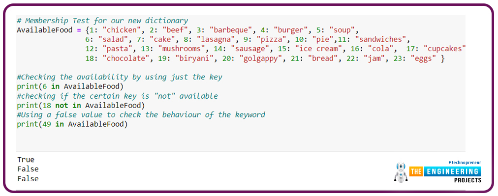
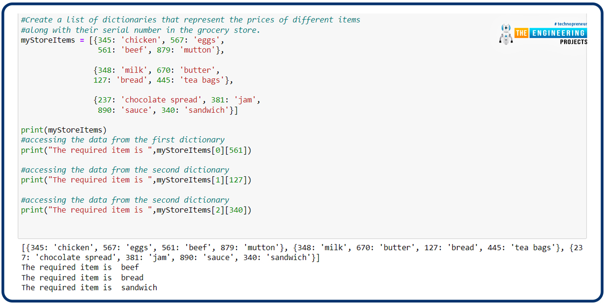
Hello peeps! Welcome to the new episode of the Python tutorial. We have been working with different types of data collection in Python, and it is amazing to see that there are several ways to store and retrieve data. In the previous lecture, our focus was on the basics of dictionaries. We observed that there are many important topics in the dictionaries, and we must know all of them to make our base of concepts solid. For this, we are now dealing with the dictionaries in different ways, and this tutorial is going to be very interesting because we will pay more heed to the practical work and, by choosing a few cases in our codes, we will apply multiple operations to them. So have the highlights of today’s learning, and then we will move forward with the concepts.
What are nested diction ...
Hello students! Welcome to the new Python tutorial, where we are learning a lot about this programming language by applying the codes in a Jupyter notebook. It is interesting to see how simple codes with easy syntax can be useful to store, retrieve, and use data in different ways. Many things in Python are so unadorned and pre-defined that programmers may use them in a productive way without any issue.
In the previous lecture, we have seen the details of the sets and how different types of mathematical operations are used to get the required results. We have seen many codes, the examples of which were taken from day-to-day life. In the present lecture, the mission is to learn a new topic that is related to the concepts of previous lectures. Yet, it is important to have a glance at t ...