Greeting learners! Welcome to the new tutorial on Python, where we are going to discuss the loops. In the previous lecture, our focus was on the primary introduction of the loops in Python. If you are from a programming background, you must know that there is a little bit of difference between the loops in Python and those in other programming languages. At the end of the previous lecture, we saw the details of the basic differences and examined why we consider Python better than other languages when considering loops. In the current lecture, our focus is only on the while loop, and you will get to know its importance soon when we discuss the detail of this loop. But before this, have a look at the list of the major concepts:
What are the loops?
Why do we use the while loop in Python?
W ...
Greetings Learners! Welcome to the new lecture on Python. Today we are moving towards an interesting and important concept. If you have come from a programming background, then you must know about the workings of loops. To make the repetition of the same sequence, we use loops. We are familiar with the sequences in detail as we have learned them in the previous lectures and have received the concept in the recent lecture. If you want to be a programmer, then you can not move forward without a solid base of loops; therefore, in this lecture, we will learn the concept of loops from scratch and then go on to a deep understanding of each loop in the next episodes. So have a look at the concepts that you will learn today.
What are the loops?
How do we understand the concept of loops from scra ...
Hi learners! Welcome to the next episode of learning the arrays using string data. We have been working with the arrays and in the previous lecture, we saw the interesting characteristics of the string arrays. In the present lecture, our target is to get knowledge about the built-in functions and we will take the strings in the array so that we may know about both of them together. String arrays are used in many officials uses and therefore, we want to use the built-in functions that every Python programmer must know. Here is the list of the concepts that will be polished in this lecture:
What are the built-in methods?
How do you differentiate between methods and functions in programming?
Give different examples to understand different built-in methods to be used in the same code.
How ...
Hola students! Welcome to the new Python tutorial, where we are learning about OOP. We all know why OOP is important in programming. In the previous lecture, a detailed overview of classes and objects was discussed. We are moving towards the next step of learning where our focus will be on inheritance. Yet, programming also contains inheritance. We have all read about inheritance in real life and are aware of the concepts surrounding it. This time, we will discuss these concepts according to the workings of the classes and related entities. The concept of inheritance is the same in both scenarios, and with the help of interesting examples, the practical implementation of inheritance will be shown to you, but first of all, it would be interesting to know about the main headings that will be ...
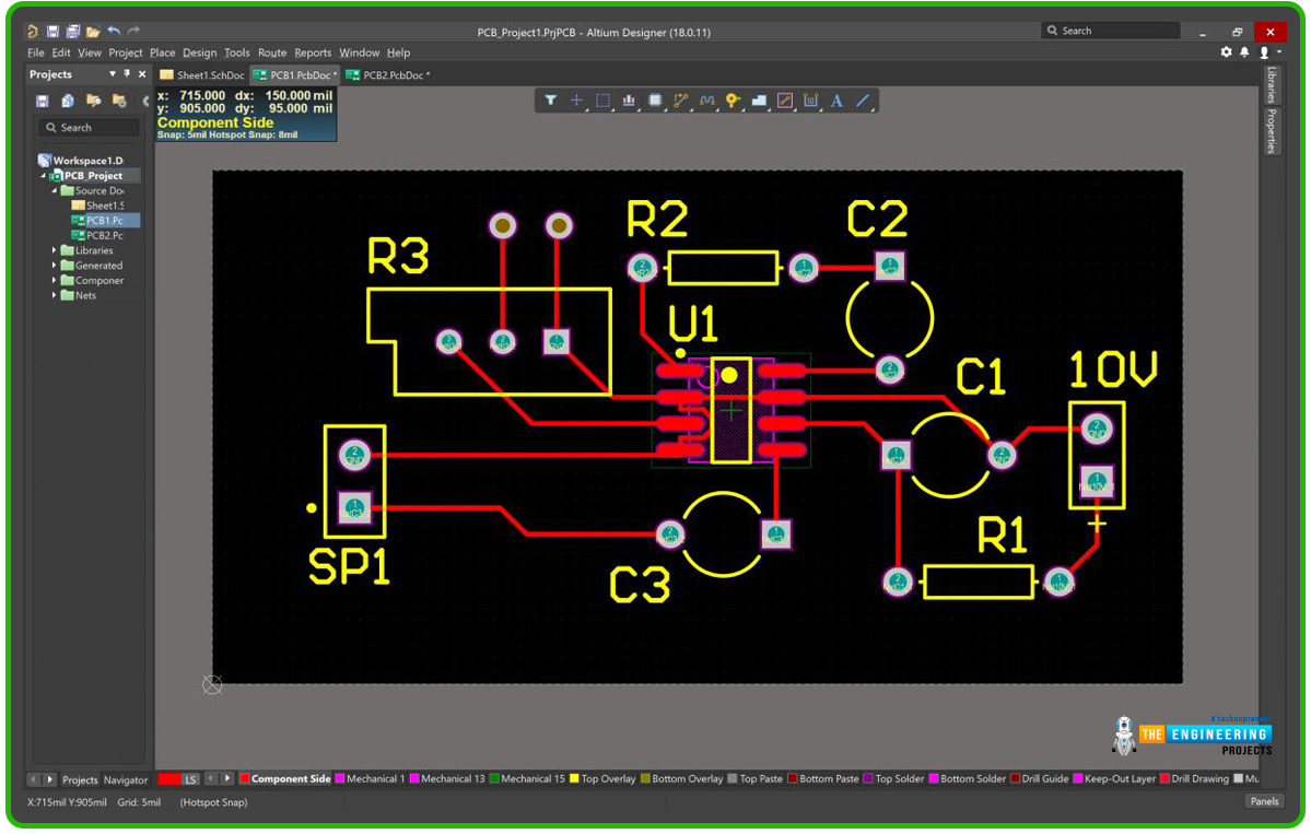
In the realm of PCB manufacturing, the Gerber file format plays an important role in the design and production processes. Understanding and inspecting these files are crucial to ensuring the accuracy and quality of the printed circuit board (PCB). JLCPCB is a leading PCB fabrication and assembly service provider. Fortunately, it offers an exceptional online tool. It is called the JLCPCB Online Gerber Viewer. It simplifies and enhances the inspection of PCB layouts. In this article, we will discuss the significance of Gerber files. We will explore the reasons for inspection. We will also showcase the powerful functionalities of JLCPCB's Online Gerber Viewer.
What is a Gerber file?
A Gerber file, named after the famous G ...
Artificial intelligence plays a crucial role in commerce by providing personalized recommendations based on previous searches and online behavior. With AI, businesses can optimize products, plan inventory, and improve logistics, which leads to reduced operating costs and increased margins. Whether you aim to scale personalized experiences, delight customers, or create new revenue streams, building an AI solution is essential. While priorities may differ among business owners, AI remains integral to implementing a variety of solutions. In this article, we discuss how AI experts can help develop and grow businesses.
What Are AI Solutions?
Artificial intelligence solutions offer pre-built or customizable options to tackle specific use cases and ...
Targeting customers and niche demographics online continues to grow in relevance as more companies adopt telecommuting practices. For this purpose, mass emailing is superior to less extensive forms of advertising in terms of both obtaining prospects and reaching the intended customer base. Amid the growth of social networking sites and other promotional channels, email marketing efforts stay at the forefront of the industry.
Using mass emailing, businesses may find valuable and potential customers for their products and services. Promoting both products and services with the help of such a service increases the likelihood of generating leads and improving ROI.
To help our readers find the easiest options for this, we have compiled a list of easy ways to send a mass email in Gmail bel ...
Hello pupil! We hope you are doing well with object-oriented programming with Python. OOP is an extremely important topic in programming, and the good thing about Python is that the concept of OOP can be implemented in it. In the previous lecture, we made a basic introduction to all the elements that are used in the OOP, and right now, we are moving forward with the detail of each concert with examples. The imperative nature of the OOP is useful for us because it uses the statements to change the programming state, and in this way, the working of the code becomes easy and effective. To use the applications of Python, the imperative nature of OOP will give us the tools we need to get the perfect results by using our creativity. We will prove this in just a bit, but here are the highlights o ...
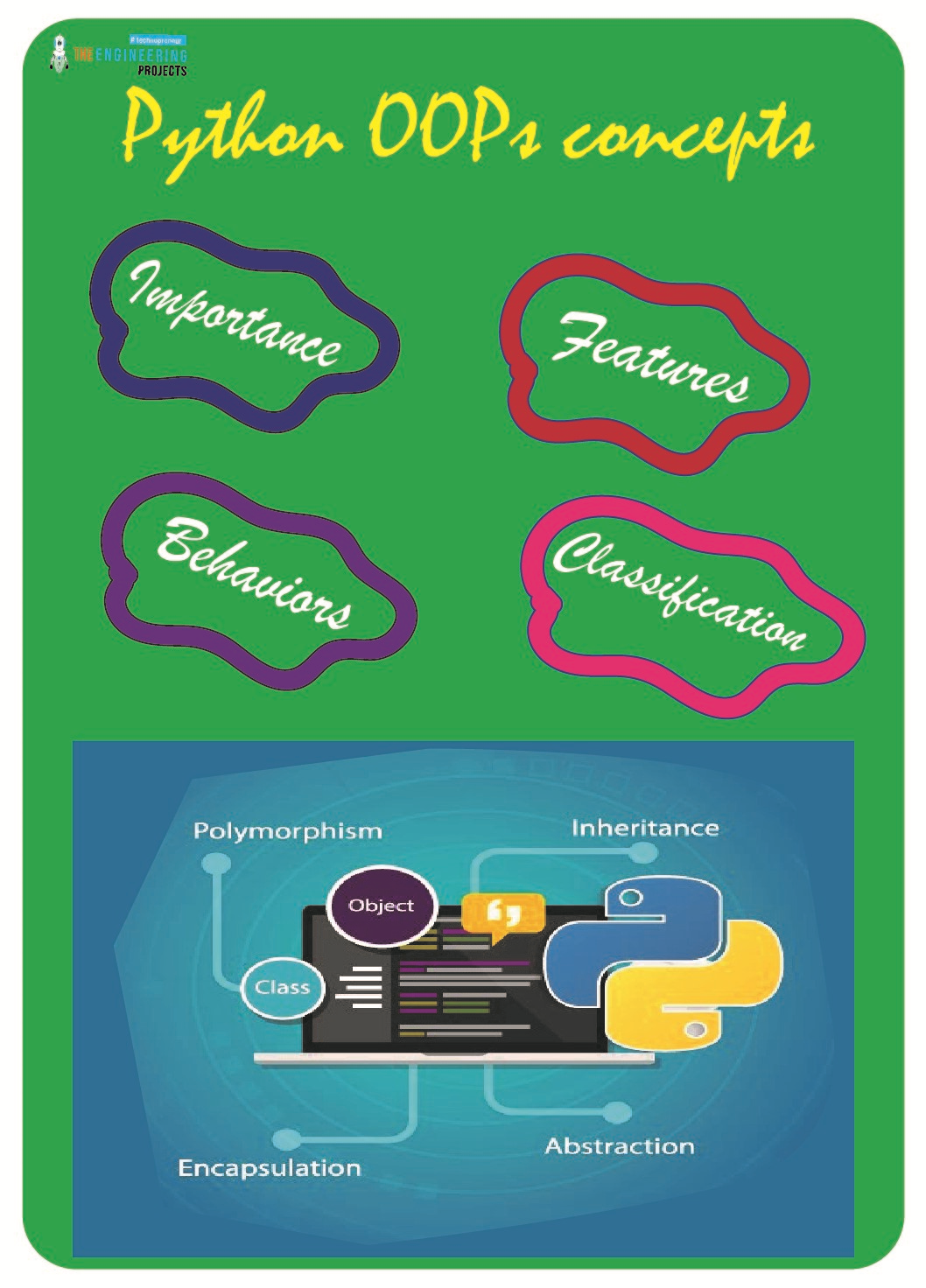
Hey peeps! Are you excited to begin with the new chapter in Python? Till now, we have been learning the data types and their related concepts. Now, we are starting a new chapter where you will learn the details of Object Oriented Programming or OOP. We are moving towards the advanced level of programming in Python, and here, you will go through the complex but interesting concepts that will show us the fascinating results on the screen. This will be more clear when you will know the basic information about the OOP, but before going deep, we will go through the headlines of the lecture:
How do you classify the programming languages?
How do you introduce the OOP?
Why object-oriented programming is important in Python?
How do you define class and objects in OOP and how are they connected? ...
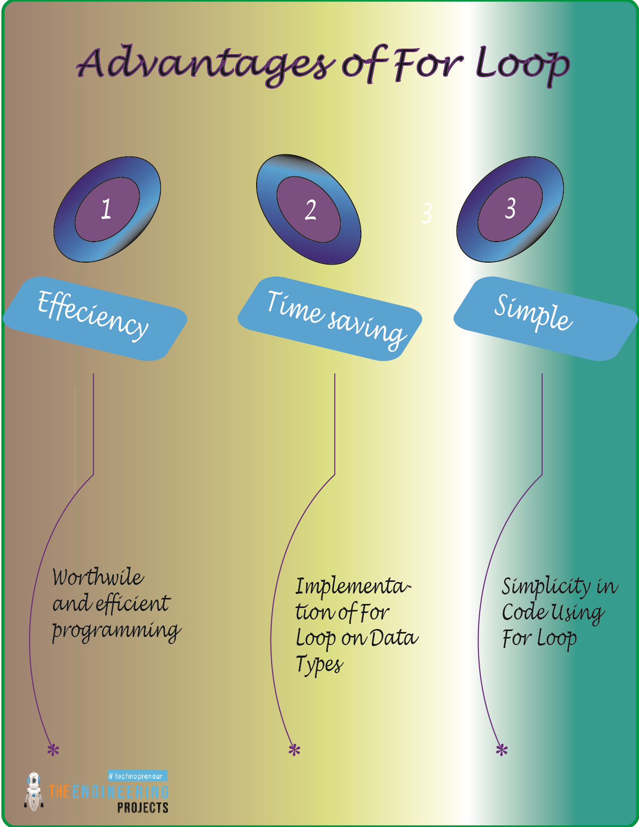
Hey peeps! Welcome to the new tutorial for the Python programming language, where we are at the point where we are going to learn about the loops. Loops are fundamental concepts in programming, and if we talk about Python, there is a smaller variety of loops in it, but the most important ones are available to practice in Python. In the last session, there was a long discussion about the while loop in detail. We had seen some examples and the details of the statements that can be used within the while loop. In the present lecture, we are going to discuss the second type of loop in Python, that is, the for loop. You will go through the training of every important and basic step about this loop, but first of all, you have to look at the basic list:
Why do we prefer for loop over some other c ...