Hi readers! I hope you are having a creative day. Today, I am sharing the list of the top embedded proteus libraries in V1.0 especially designed for engineering students. Till now, you have seen blogs on different projects, components, libraries, and simulations. Yet, I am sharing the list of the first versions of these embedded libraries that will help the students throughout multiple projects. These libraries are highly useful in multiple domains of engineering, and if you don’t know how to download the new libraries
, then you must see the link provided.
This is the list of all new proteus libraries for engineering students
. The zip files are present in the link to the related manual, which has details on how to download, install, and use these libraries. Now, let’s start learning ...
Hi readers! I hope you are doing great. Today, I am going to share the second version of the top embedded libraries designed for the proteus. Before this, we shared the first version of many libraries that engineering students are using in their projects. The interest of the students in these libraries has motivated us to design even better versions of them. These versions have a more realistic design and error-free working and are ideal for engineering students to use in their simulation in Proteus.
If you don’t know how to download and use these libraries, then you must learn how to add a new library in Proteus
. Moreover, if you are interested in learning the details of all the libraries, you must see the new proteus libraries for engineering students
. The installation and app ...
In the realm of online entertainment and gaming, 1xBet Bingo Online emerges as a shining star, offering a captivating and immersive experience for players of all backgrounds. As a team of seasoned SEO and copywriting experts, we are here to delve deep into the world of 1xBet
Bingo Online, uncovering its hidden gems, unique features, and what sets it apart from the competition. Buckle up as we embark on this thrilling journey!
A World of Bingo at Your Fingertips
1. The Ultimate Bingo Destination
At 1xBet Bingo Online, you're not just playing bingo; you're immersing yourself in a vibrant and dynamic bingo community. With a wide array of bingo rooms catering to all tastes and preferences, you can experience the thrill of the game like never before. From traditional 75-ball and 90-ball ...
The digital age has ushered in a new era of computing, and at the core of this transformation is cloud computing. Whether you're sending emails, streaming videos, or running a global enterprise, there are high possibilities you're already benefiting from the power of the cloud. For those venturing into the dynamic field of cloud computing or striving to sharpen their expertise, the right book can be an invaluable guide. I have benefitted from many books that throw light on the fundamentals of cloud computing, making the dynamic field of cloud computing interpretable and accessible.
This article is your guide to the finest cloud computing books, carefully curated to direct both beginners and seasoned individuals in the field. Read on to explore these literary companions that illustra ...
When embarking on a new project, whether it's a construction job, a manufacturing operation, or even a simple office renovation, procuring the right equipment and supplies is crucial for its success.
However, the process of acquiring these essentials involves more than just placing orders - you need to deal with multiple hurdles before you get the equipment you need, right from buying quality materials that are affordable to transferring these materials to the place of the project.
To ensure a smooth and efficient project, you need to pay close attention to various logistics aspects. In this blog, we'll explore eight important logistics considerations when buying new equipment and supplies for your project.
1. Assess Your Project Needs
Before you even start shopping for equipment a ...
Experiencing water damage to your ceilings can feel like a setback. It's a situation no homeowner wants to contend with. Yet, timely action can mitigate the damages and save you from costly repairs.
This handy guide presents steps detailing what you can do when your ceiling has suffered water damage, starting from spotting the initial signs to navigating insurance claims. We'll also shed some light on how professional water damage companies could be your best bet in resolving the issue efficiently and effectively.
Let me guide you on this journey to reclaiming your safe and dry living space.
1. Identifying Water Damage on Your Ceilings
The sooner you notice potential water damage, the quicker and more efficient the treatment process can be. Therefore, a proactive approach is your b ...
Sometimes you may be asked to submit a written piece of note in the form of handwriting. We all know, writing by hand is quite a labor-intensive and time-consuming task. You first have some blank pieces of white paper, and then find the required information from an online source. After this, the writing process will start.
So, what’s the solution to this? Fortunately, there is a quick and effective solution available. If you are asked to convert some pieces of text available online into handwritten notes, then instead of manually noting it down, you can consider utilizing text-to-handwriting tools.
These tools allow users to convert normal text into handwritten style in real-time.
Remember, utilizing online tools is the only solution if you don’t want to make use of pe ...
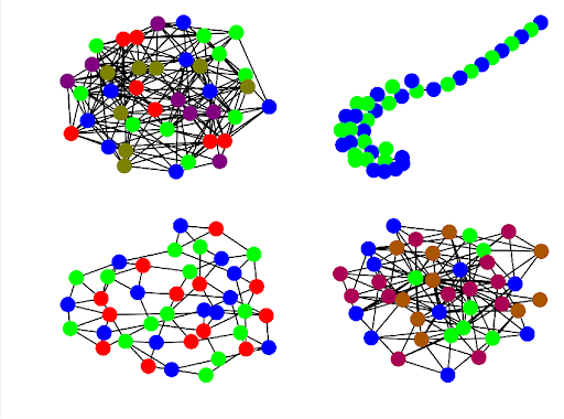
Hi readers! I hope you are doing great. We are learning about modern neural networks in deep learning, and in the previous lecture, we saw the capsule neural networks that work with the help of a group of neurons in the form of capsules. Today we will discuss the graph neural network in detail.
Graph neural networks are one of the most basic and trending networks, and a lot of research has been done on them. As a result, there are multiple types of GNNs, and the architecture of these networks is a little bit more complex than the other networks. We will start the discussion with the introduction of GNN.
Introduction to Graph Neural Networks
The work on graphical neural networks started in the 2000s when researchers explored graph-based semi-supervised learning in the neural network. The ...
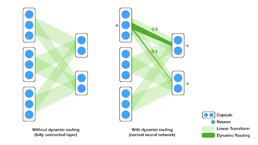
Hey pupil! Welcome to the next lecture on modern neural networks. I hope you are doing great. In the previous lecture, we saw the EffcientNet neural network, which is a convolutional Neural Network (CNN), and its properties. Today, we are talking about another CNN network called the capsule neural network, or CapsNets. These networks were introduced to provide the capsulation in CNNs to provide better functionalities.
In this article, we will start with the introduction of the capsule neural network. After that, we will compare these with the traditional convolutional neural networks and learn some basic applications of these networks. So, let’s start learning.
Introduction to Capsule Neural Networks
Capsule neural networks are a type of artificial neural network that was introduc ...
The last decade brought about a lot of advancements that we didn’t think would even be possible. In the case of business communication, the biggest benefit next to the internet is VoIP. Thanks to this technology, all business owners (even those whose budgets are extremely meager) can set up a strong communication system on par with their more established counterparts.
But when talking about how helpful VoIP can be, the conversation is always focused on calls. People always talk about how Telnum and other telecom providers are able to slash their phone bills, enhance the communication features they enjoy, and many more.
What about SMS? Unfortunately, the advantages in this area are unknown to many users. There are so many benefits If you want to fully harness the capabilities that are ass ...