
Autoencoders as Masters of Data Compression


Hey readers! Welcome to the next episode of training on neural networks. We have been studying multiple modern neural networks and today we’ll talk about autoencoders. Along with data compression and feature extraction, autoencoders are extensively used in different fields. Today, we’ll understand the multiple features of these neural networks to understand their importance.
In this tutorial, we’ll start learning with the introduction of autoencoders. After that, we’ll go through the basic concept to understand the features of autoencoders. We’ll also see the step by step by step process of autoencoders and in the end, we’ll see the model types of autoencoders. Let’s rush towards the first topic:
What are Autoencoders?
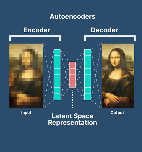
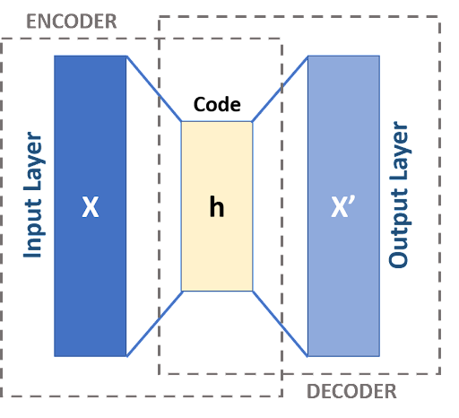
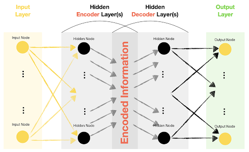
Autoencoders are the type of neural networks that are used to learn the compressed and low-dimensional representation of the data. These are used for unsupervised learning and are particularly used in tasks such as data compression, feature learning, generation of new data, etc. These networks consist of two basic parts:
Encoders
Decoders
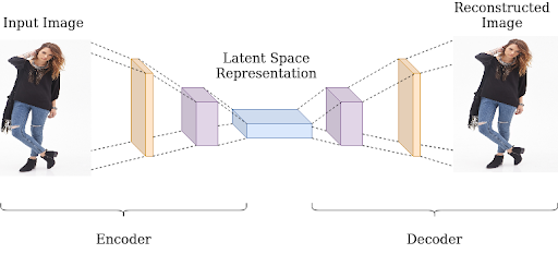
Moreover, between these two components, it is important to understand the latent space that is sometimes considered the third part of the autoencoders. The goal of this network is to train and reconstruct the input data at the output layer. The main purpose of these networks is to extract and compress the data into a more useful state. After that, they can easily regain the data from the compressed state.
Basic Concepts to Understand Autoencoders
The following are some important points that must be made clear when dealing with the autoencoder neural network:
Encoders in Autoencoder Neural Network
This is the first and most basic component of the autoencoders. These are considered the heart of autoencoders because they have the ability to compress and represent the data. The main focus of encoders is to map the input data from high dimensional space to low dimensional space. In this way, the format of the data is changed to a more usable format. In other words, the duty of encoders is to distill the essence of the input data in a concise and informative way.
Autoencoders Latent Space
The output of the autoencoders is known as latent space. The difference between the latent space and the original data is given here:
Dimensions of Data
The dimension of the data is an important aspect of neural networks. Here, the dimensions are smaller and more compact than in the original data. Choosing the right dimension is crucial for efficient representation and detail in getting the details of the data.
Structure of the Latent Space
The structure of the data from encoders (latent space) has information about the relationship between data points. These are arranged in such a way that similar data points are placed closer to each other and dissimilar data points are far apart. This type of spatial arrangement helps in the efficient retrieval and arrangement of the data in a more efficient way.
Feature Extraction in Latent Space
Feature extraction is an important point in this regard because it is easier with the latent space data than with the normal input data fed into the encoders. Hence, feature extraction is made easy with this data for processes like classification, anomaly detection, generating new data, etc.
Decoders in Autoencoders
The decoder, as the name suggests, is used to regenerate the original data. These take the data from the latent space and reconstruct the original input data from it. Here, the pattern and information in the latent space are studied in detail and as a result, closely resembling input data is generated.
Generally, the structure of encoders is the mirror image of the encoders in reverse order. For instance, if the architecture of the encoders has convolutional layers, then the decoders have deconvolution layers.
During the training process, the decoder’s weight is adjusted Usually, the final layer of the decoders resembles the data of the initial layer of the input data in the encoders. It is done by updating and maintaining the weights of the decoders corresponding to the respective encoders. The difference is that the neurons in the decoders are arranged in such a way that the noise in the input data of the encoders can be minimized.
Steps in the Training Process of Autoencoders
The training process for the autoencoders is divided into different steps. It is important to learn all of these one by one according to the sequence. Here are the steps:
Data Preparation in Autoencoders
The data preparation is divided into two steps, listed below:
Gathering of the Data
The first step is to gather the data on which the autoencoders have to work. For this, a dataset related to the task to be trained is required.
Autoencoders Preprocessing
The preparation of the data required initial preprocessing. It requires different steps, such as normalization, resizing for images, etc. These processes are selected based on the type of data and the task. At the end of this process, the data is made compatible with the network architecture.
Autoencoders Model Architecture
There are multiple architectures that can be used in autoencoders. Here are the steps that are involved in this step:
Selecting the Appropriate Architecture
It is very important to select the right architecture according to the datasets. The encoder architecture aligns with the data type and requirements of the task. Some important architectures for autoencoders are convolutional for images and recurrent for text.
Autoencoders Network Layers Specifications
In the same step, the basic settings of the network layers are also determined. Following are some basic features that are determined in this step:
Determination of the number of layers in the network
Numbers of neurons per layer
Suitable activation functions according to the data (e.g., ReLU, tanh).
Autoencoders Training Loops
The training is the most essential step and it requires great processing power. Here are the important features of the autoencoders:
Autoencoders Feed Forward
In this step, the processing of the input data is carried out. The data is sent to the encoder layer, which generates the latent representation. As a result of this, latent space is generated.
Decoder Reconstruction
The latent space from the encoder is then sent to the decoder for the regeneration of the input data, as mentioned before.
Autoencoders Output Calculation
Here, the decoders’ output is then calculated with the original input. Different techniques are used for this process to understand the loss of data. This step makes sure that the accurate data loss is calculated so that the right technique is used to work on the deficiencies of the data. For instance, in some cases, the mean squared error for images is used and in other cases, categorical cross-entropy for text is used to regenerate the missing part of the data.
Autoencoders Backpropagation
Backpropagation is an important process in neural networks. The network propagates backward and goes through all the weights to check for any errors. This is done by the encoders as well as by the decoders. The weights and bosses are adjusted in both layers and this ensures the minimum errors in the resultant networks.
Autoencoders Optimization
Once the training process is complete, the results obtained are then optimized to get an even better output. These two steps are involved here:
Choosing the Right Optimizer
Different cases require different types of calculations; therefore, more than one type of optimizer is present. Here, the right optimizer is used to guide the weight update. Some famous examples of optimizers are Adam and stochastic gradient descent.
Autoencoders Learning Rate Adjustment
Another step in the optimization is the learning rate adjustment. Multiple experiments are done on the resultant output to control the learning speed and avoid overfitting the data in the output.
Autoencoders Regulation
This is an optional step in the autoencoders that can prevent overfitting. Here, some different techniques, such as dropout and weight decay, are incorporated into the model. As a result of this step, the training data memorization and improvement of the generalization of the unseen data are seen.
Autoencoder Monitoring and Evaluation
The getting of the results is not enough here. Graduation monitoring is important for maintaining the outputs of the neural networks. Two important points in these steps are explained here:
Tracking Training Process
During the training process, different matrices are assessed to ensure the perfect model performance; some of these are given here:
Monitor reconstruction loss
Checking for the accuracy of results
Checking the rate of precision
Recalling the steps for better performance
The evaluation process is important because it ensures that any abnormality in the processing is caused during its initial phase. It stops the training process to prevent any overfitting of the data or any other validation.
Autoencoders Models
The autoencoders have two distinct types of models that are applied according to the needs of the task. These are not the different architectures of the data but are the designs that relate to the output in the latent space of the autoencoders. The details of each of these are given here:
Under-complete Autoencoders
In under-complete autoencoders, the representation of the latent space dimensions is kept lower than the input space. The main objective of these autoencoders is to force the model to learn all the most essential features of the data that are obtained after the compression of the input. This results in the discovery of efficient data representation and, as a result, better performance.
Another advantage of using this autoencoder is that it only captures the rare and essential features of the input data. In other words, the most salient and discriminative data is processed here.
Dimensionality Reduction in Under-complete Autoencoders
The most prominent feature of this autoencoder is that it reduces the dimensions of the input data. The input data is compressed into a more concise way but the essential features are identified and work is done on them.
Under Complete Autoencoders Applications
The following are important applications of this model:
The main use for an under-complete autoencoder is in cases where compression of the data is the primary goal of the model. The important features are kept in compressed form and the overall size of the data is reduced. One of the most important examples in this regard is image compression.
These are efficient for learning the new representation of the efficient data representation. These can learn effectively from the hierarchical and meaningful features of the data given to them.
Denoising and feature extraction are important applications of this autoencoder.
Over Complete Autoencoders
In over-complete autoencoders, the dimensions of the latent space are intentionally kept higher than the dimensions of the latent space. As a result, these can learn more expressive representations of the data obtained as a result. This potentially captures redundant or non-essential information through the input data.
This model enables the capture of the variation in the input data. As a result, it makes the model more robust. In this case, redundant and non-essential information is obtained from the input data. This is important in places where robust data is required and the variation of the input data is the main goal.
Feature Richness
The special feature of the autoencoder is its feature richness. These can easily represent the input data with a greater degree of freedom. More features are obtained in this case that are usually ignored and overlooked by the undercomplete autoencoders.
Applications of Overcomplete Autoencoders
The main applications of overcomplete autoencoders are in tasks where generative tasks are required. As a result, new and more diverse samples are generated.
Another application to mention here is representation learning. Here, the input data is represented in a richer format and more details are obtained.
Hence, today, we have seen the important points about the autoencoders. At the start, we saw the introduction of the autoencoders neural networks. After that, we understood the basic concepts that helped a lot to understand the working process of autoencoders. After that, we saw the step-by-step training of the autoencoders and in the end, we saw two different models that are adopted when dealing with the data in autoencoders. We saw the specific information about these types and understood the features in detail. I hope this is now clear to you and this article was helpful for you.


 1 user


 Continue Wishlist


 Getting Started Guide
 Help Center
 Contact us
 Doist Blog
 Privacy
 Security
 Terms of Service
 What's new: Channel Descriptions


 Deep Learning
 xeohacker
 0 Comments



 Autoencoders as Masters of Data Compression
deep learning autoencoders
 Monday, January 8, 2024