Step Response of an LTI System in MATLAB

Hey readers, welcome to another interesting lecture of this series in which we are studying signals and systems. In the present lectures, we are learning the details about the responses of LTI systems, and today, you are going to learn the step response. We also talked about the impulse response and frequency response, and therefore, this lecture will be easy for you to understand because it is, somehow, related to the impulse response. If you are new to this concept, do not worry because there will be a revision of important points side by side. Have a look at the list of today’s concepts:

• What is an LTI system?

• How do you define the step response of an LTI system?

• What is the code to run the step response of signal in MATLAB using different functions?

• How can you find the detail of the graph of the step response?

• What is the difference between step response and impulse response?

We are going to learn each of them in detail so that if you know any of these already, you may have a revision about the topic.

What is the LTI System?

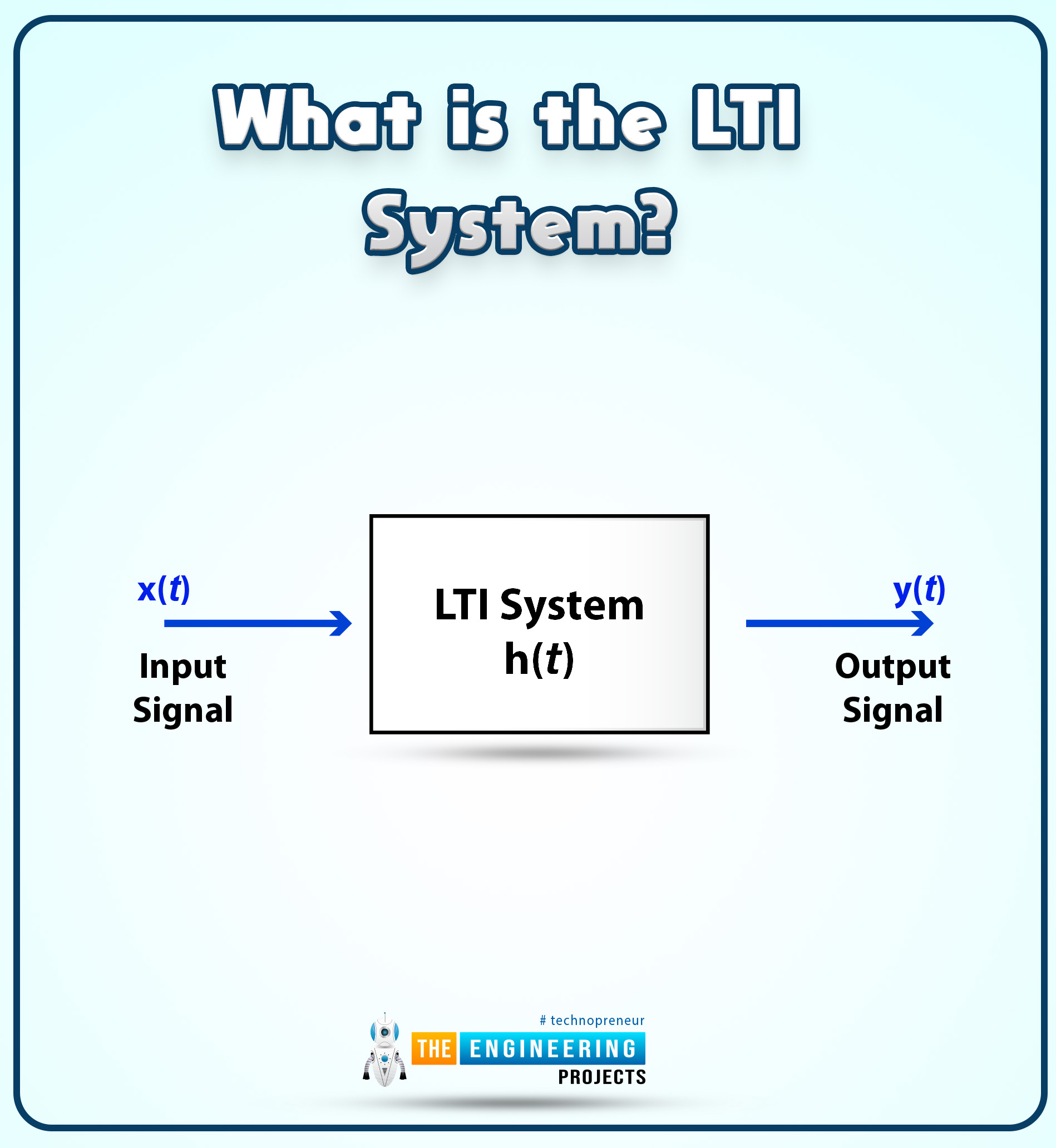
We all understand that a system is something that receives input at one end and produces output at the other end after performing specific operations on the input. We define the LTI system as follows when discussing it:

The term "linear time-invariant system," or "LTI system," refers to a system that simultaneously possesses both linearity and the time-invariant property.

So, keeping this in mind, we are going to discuss the whole concept of a step response in the LTI system. Refresh the definition of convolution in your mind so that it says convolution is the process in which two signals are overlapped in such a way that they form a third signal. So, keeping in mind the above image, we can use this concept to define the step response of the LTI system. 

What is the Step Response of the LTI System? 

First of all, let us clear that step signals are the one whose values always lies in just positive time and for the negative time, these signals does not have any value. The unit step signals are usually denoted as u(t). So, mathematically, we can say the step step signals are formed with the value only when t> = 0, and for t<0, signals do not exist. In this way, we get the signal at the right area of the graph, that is, the positive side values of the time. By the same token, the step response is the behavior of the LTI system when the input is provided in the form of a step signal and the output then depends upon the integral of the impulse response of that LTI system. We’ll see the proof of this statement in just a bit, but prior to that, have a look at the definition of step response:

“The step response of an LTI system is obtained when the input provided to the system is unit step and, therefore, the output also has similar characteristics.”

Using all this information, we can derive the formula for step response:

s(t)=h(t)∗u(t)

Where:

s(t)= step response

h(t) = impulse response

u(t)=unti step response 

Then,

S(t) = H(t). U(t)

S(t)=(1/t).U(t)

Now, applying the inverse Laplace transform to the equation given above, we get:

s(t)=∫h(t).d(t)

So this is the final formula that is used to calculate the value of the unit step function in an LTI system. You must know that here h(t) is the impulse response of the system that we also have read in detail in the previous session. You can have stronger concepts if you examine the example that we are going to discuss in the next section. 

Step Response in MATLAB

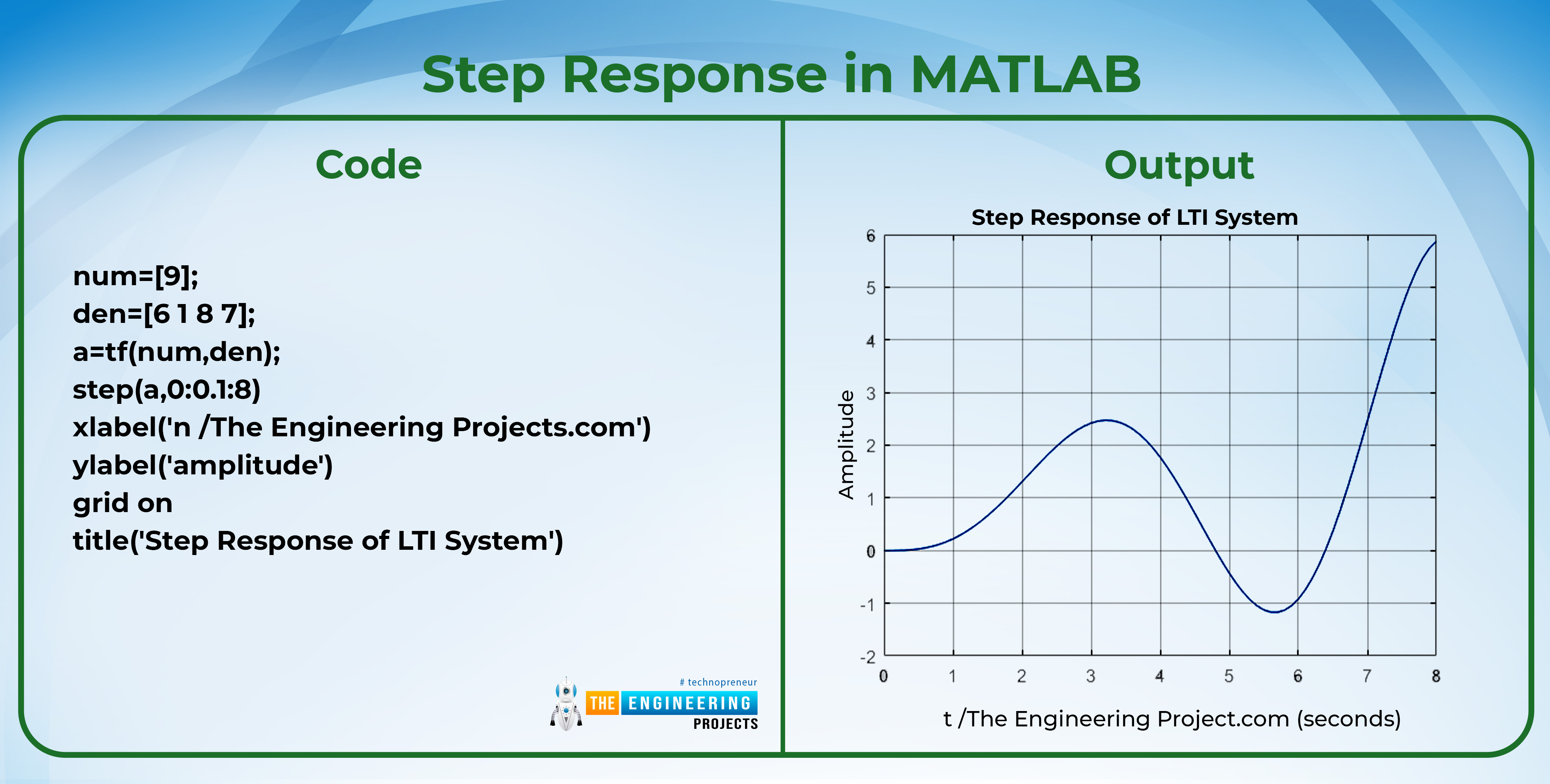
Code

num=[9];

den=[6 1 8 7];

a=tf(num,den);

step(a,0:0.1:8)

xlabel('n /The Engineering Projects.com')

ylabel('amplitude')

grid on

title('Step Response of LTI System') 

Output:

There are some functions that are used here but are new to you. So, have a look at the details of each of them and then try to understand the code.

The Transfer Function in MATLAB

It is an important function in MATLAB that gives us the facility to have the same results by using this function instead of using many lines of code. Using this function, we can represent the numerator and denominator in polynomial form. The syntax of this function is

y=tf(num, den)

where num and den are specified before using this function. These are the numerator and denominator in descending power of s and are in the form of a polynomial. For example, in the code given above, the equation we used is

9/6(s)^3+1(s)^2+8s+7

Before the introduction of this function in this series, we used different and relatively complex calculations in the code to achieve the same results. In short, this function has made our work simpler. 

Step Function in MATLAB

MATLAB has a built-in function step that is used to get the step response of an LTI system. The syntax of the step function is given as:

step(x,y)

Where 

x = the equation whose step function is required.

y = the time interval of the step function.

Usually, the equation is in the form of a polynomial and it is pre-defined when this function is called. You can also use the variable in which the time interval is stored before using it. Yet, we have used the exact time interval so that you may have the concept of doing so. 

How the Program of Step Response Worked at MATLAB

• First of all, we have declared the values of the polynomials of the numerator and denominator and stored them in the variables num and den, respectively. 

• We have used the transfer function to convert these values into a polynomial equation and then saved the result into the variable a to use later. 

• Next, we used the step function and put all the required values in it. 

• Notice that we have not used the stem or plot function to represent the results in the graphical format. We have just used the labels on the graph. It means the step function itself provides you with the information in a graphical format. 

• Another thing to notice is the visibility of the text “Second” on the time axis of the graph. We have not used it in the x-label but it is automatically defined in the step function. 

How to Examine Step Response in MATLAB

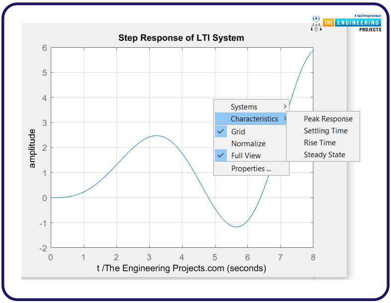
Here is an interesting thing about the step response. You can directly examine the graph by following some simple steps. 

• Write the code in the editor window. 

• Run the code

• Provide the path and save the program. 

• A graph will appear as shown in the code given above. 

• To examine it clearly, left click on the graph. 

• Different options will appear on the screen. Hover the mouse over the characteristics. 

• You can tick the feature on the graph you want and can choose more than one at a time. 

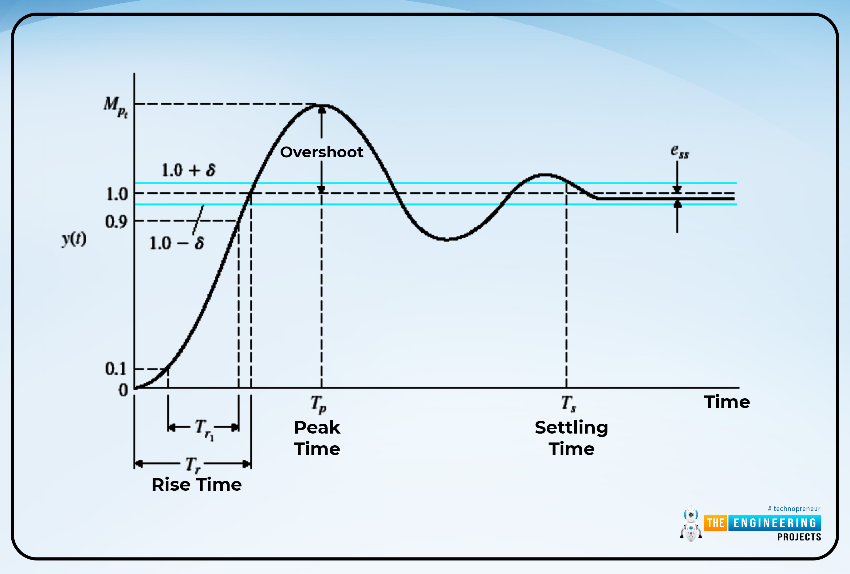
• Once you follow the step given above, you will get the details according to the graph. A great overview of the graph is given in the image given below:

Let’s understand what is going on the each step and why these terms are labeled so. 

Overshoot

In the graph of step response, overshoot is the area that shows the highest bump in the graph. Basically, it shows that values that are shot over the targeted values, which is why it is named so. At its start, the values indicate the values are exceeded to their steady state and at their end, the values indicate the transition from different values. 

Rise Time of Step Response

The rise time in the graph of the step response is the area that indicates the time required by the step response to reach 10%-90% of the final value to bring the system to a condition called overdamped. It also indicates the time limit when the system takes the time to reach 0%-100% to meet the underdamped condition. 

Peak Time of Step Response

The peak time of the step response is the specific value of time in the graph of step response when the overall response of the system reaches its maximum position. Usually, you can see that it is the peak value of the graph. 

The Settling Time of Step Response

The response's settling time is the amount of time needed to calm oscillations and maintain a 2% to 5% error (or tolerance) band from its final value.

So, in this way, you can understand what is going on in the step response. It is a common question how the step response is different from the impulse response because the basics of both of them are similar and why do we find both of them in the signal? 

Difference Between Step and Impulse Response

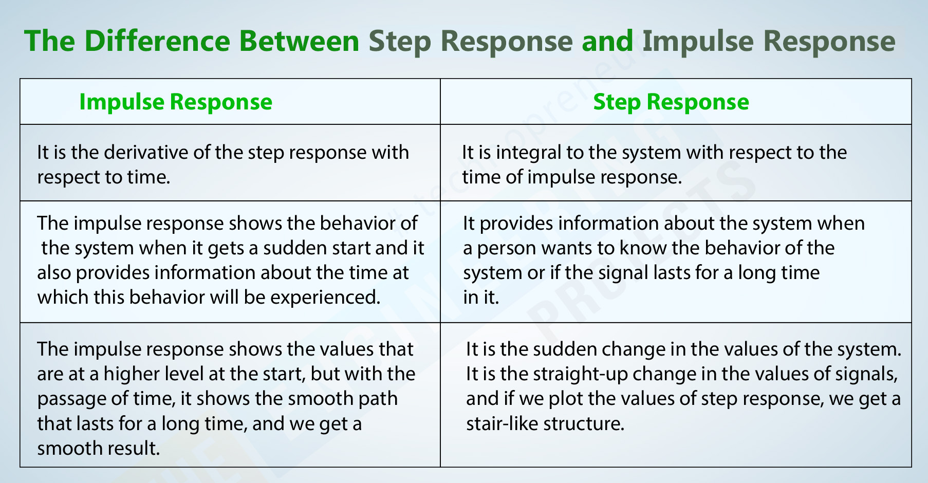
Many times, when dealing with the signal, people are confused between these two because of the similarity in the system and some other resembling features. Therefore, we have made a comparison between these two, and here are some important points about them.

Why Do We Use Step Response in LTI Systems?

There are several cases where it is more useful to have the step response over the other types of response. Some of the major reasons are listed below:

1. The step response is used because it does not require information about the dynamics of the system; hence, it can be run with the help of less information. 

2. If we have the values of the step response, we can find the impulse response by simply differentiating the step response. In this way, we can solve the system even if we do not know the initial condition. 

3. It is important to notice that integration has noise rejection characteristics, and we have discussed before that step response is the inherited integral of the impulse response. 

In this lecture today, we have read a large piece of information about the step response. To have a solid foundation for the topic, we have to refresh the concept of the linear time-invariant system and the step signal in our minds. Moreover, we have also seen the example of step response in MATLAB. For a clear idea, we also read a detailed description of each function used in the code, and then we read about the flow of the program in MATLAB. In the end, we read the details of different terms used during the examination of step response and also differentiate between step response and impulse response. In the next lecture, we will learn more about MATLAB and signals. To learn more, be with us. Till then, have a nice day.