
Responses of Discrete Time Signals in MATLAB


Hello learners, welcome to another topic of signals and systems. We hope you are having a reproductive day and to add more information in the simplest way to your day, we are discussing the responses in discrete-time signals. If you do not get the idea of the topic at the moment, do not worry because we are going to learn it in detail and you are going to enjoy it because we are making interesting patterns in MATLAB as the practical implementation of the topics. Have a look at the points that we are making clear today.
What is the LTI system?
What is impulse response?
How can we get the impulse response in MATLAB?
How can we have the output signal using codes and impulse response in MATLAB?
As we have learned so far in this series, there are two types of signals based on the shape of the signal we obtain, and these are
Discrete-time signals
Continuous-time signals
The focus of our topic is discrete-time signals in which the points of the signals are not connected with each other, but we get a line for each point in the graph, and in this way, we get a non-continuous wave. There are different types of operations that can be performed on discrete-time signals to get useful results from them. The types of operations that we are going to discuss on discrete-time signals are
Impulse Response
Frequency Response
Both of them are simple yet different from each other, and we are going to discuss all the necessary details about the impulse response in the next section. But to make a solid foundation, let us first define the LTI system.
What is an LTI System?
We have read about the types of systems at the beginning of this course, and we know that:
“The LTI system, or the linear time-invariant system, is those which have both characteristics at the same time, that is linearity and the time-invariant property."
We are now moving towards the introduction of the impulse response.
Impulse Response in DT Signals
Recalls that a system is something in which we provide the input at one end of the system, the operations in the system take place on the input, and from the other end of the system, we get the output.
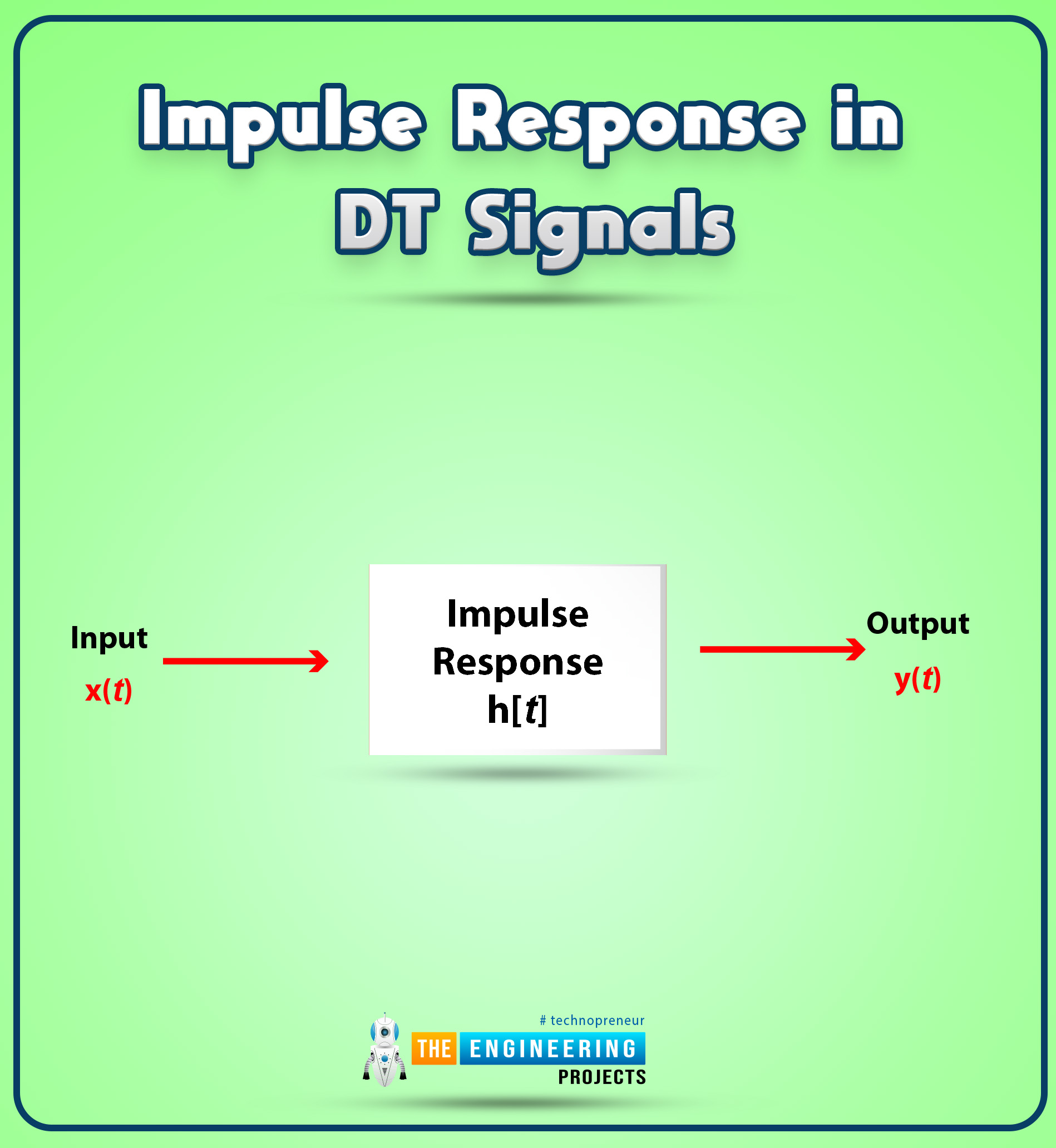
Now coming towards the impulse response, it is the procedure or the operation that is implemented on the discrete time signal and after the application of this signal, we get the required output. To clarify this statement, have a look at the image given below:
The impulse response here is the procedure that converts the input into the required output. When calculating the result theoretically, we use the mathematical form of this image.
x[t]=h[t] * y[t]
Considering the equation given above, we see that it is in the form of a time domain, and if we want to change it into a frequency domain, then we are using the Laplace transform (if you don't know it, recollect from the previous lectures).
L(x[t])=(h[t] * y[t])
Y(s) =X(s). H(s)
And in this way, we can also change the form of the equation to get the required quantity.
Y(s) =X(s). H(s)
Or
H(s)=Y(s)/X(s)
So, in this way, we can calculate the impulse response of the discrete-time signals. The H(s) here is called the transfer function, and these are used interchangeably. When we use the function in the time domain, we call it an impulse response, and in the case of the s-domain, we call it the ratio of input and output transfer function. Both of these are used for the LTI system.
While performing the transform, the signal from the time domain to the frequency domain, you can also use the other forms of transforms as well, if you do not want to use the Laplace transform. The other two types of transform that we already know are
Z transform
Fourier transform
Impulse Response in MATLAB
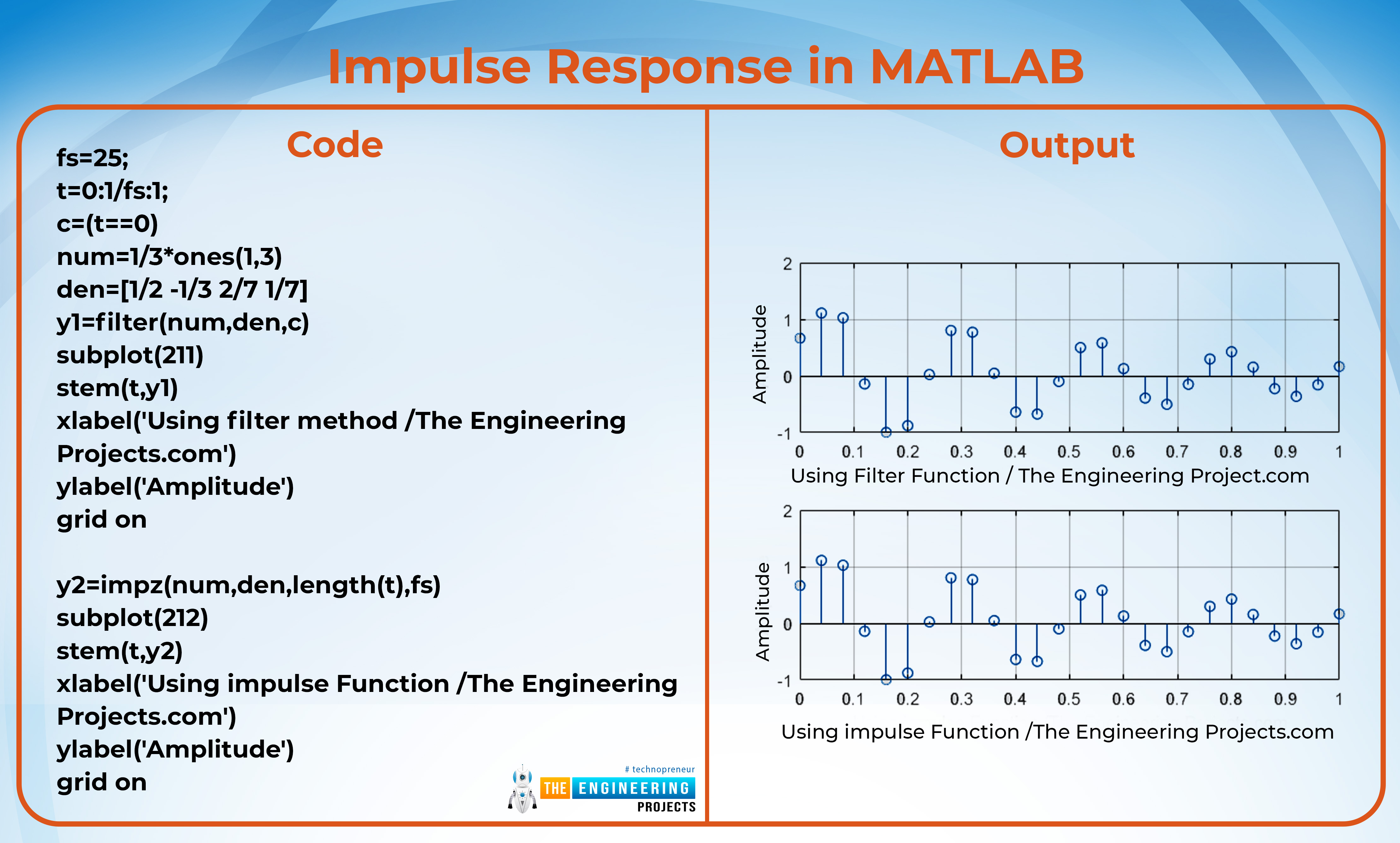
Once you know the basic definition of the impulse response, you might be interested in the example. We are describing the two methods to perform the impulse response and instead of making two different programs, we are merging them into one. Suppose we want to perform the impulse response operation with the equation given below:
½(y[n]-⅓[y-1]+2/7[y-2]+1/7[y-3]=(x[t]+x[x-1]+x[x-2])/6
Have a look at the program and if it confusing for you at the moment, do not worry, we are going to discuss it in just a bit.
Code:
fs=25;
t=0:1/fs:1;
c=(t==0)
num=1/3*ones(1,3)
den=[1/2 -1/3 2/7 1/7]
y1=filter(num,den,c)
subplot(211)
stem(t,y1)
xlabel('Using filter method /The Engineering Projects.com')
ylabel('Amplitude')
grid on
y2=impz(num,den,length(t),fs)
subplot(212)
stem(t,y2)
xlabel('Using impulse Function /The Engineering Projects.com')
ylabel('Amplitude')
grid on
Output:
Filter (b,a,x) function in MATLAB
The function of a filter is used to apply the digital filters to the equation with the values that are stored in the num and den. We all know that when dealing with the equations representing a signal, the ideal format is the one in which the values of the variable y are on one side of the equation and the values of the x variable are on the other side of the equation. So keep this point in mind and look at the representation of the signal. The syntax of this function is given next:
d= filter(b, a,x)
Where:
d= variable in which the result is stored
a = values with the x
b = values with the y
c = time
Impulse Response Function in MATLAB
There is a built-in function in MATLAB to perform the impulse function, and you do not have to do much work to perform it. It will be clear with the help of the following syntax:
impx(b,a, l, f)
Where:
b=values with y
a = values with x
l= length of the time duration
f=frequency of the signal
We have to declare the variables first and then just use them in the formula. We have used this formula in the code, and you will get the concept of working when you will learn the flow of this code. So let’s try to understand the whole code.
In the first part, we are providing the frequency with which we want to produce the output.
The time here is from 0 to 1, and the interval is the inverse of the frequency that we specify. We all know that frequency is the inverse of time.
The equation is presented as a numerator and a denominator.
In the first part, we are using the method of filtering.
In the second part of the code, the built-in impulse function is used and here we have to specify the length of the x that depends upon the time period of the signal that is specified by us in the code.
After applying the values in the function, just use the stem function and the results are here in front of you.
You can compare the results in the code. Both methods produce the same output, and it is now totally up to you which type of method you prefer to solve your impulse response problems. Your homework is to look at the numerical values that are present in the command window and the workspace area to get the concept of the graph represented.
The Output of Impulse Response in MATLAB
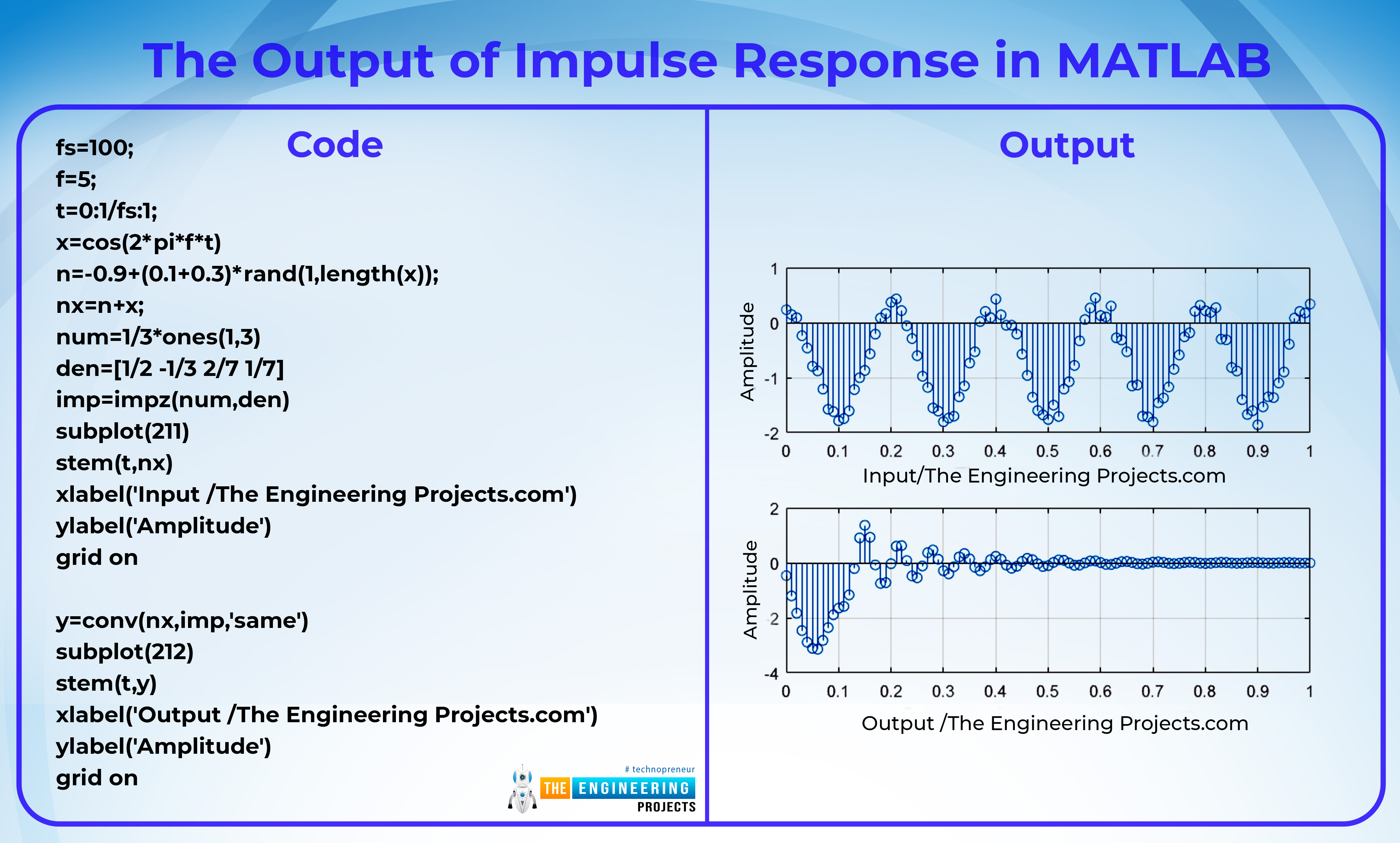
Now moving towards an interesting concept. Keeping this in mind, we can reverse the whole procedure easy to get the output of the system. At the start of this lecture, we said that by the convolution of impulse response and the input, we get the output. Let's look at this statement in action with the help of this code.
Code:
fs=100;
f=5;
t=0:1/fs:1;
x=cos(2*pi*f*t)
n=-0.9+(0.1+0.3)*rand(1,length(x));
nx=n+x;
num=1/3*ones(1,3)
den=[1/2 -1/3 2/7 1/7]
imp=impz(num,den)
subplot(211)
stem(t,nx)
xlabel('Input /The Engineering Projects.com')
ylabel('Amplitude')
grid on
y=conv(nx,imp,'same')
subplot(212)
stem(t,y)
xlabel('Output /The Engineering Projects.com')
ylabel('Amplitude')
grid on
Output:
Isn’t it interesting? We have used the same equation and we can get the required results by using some different functions of MATLAB. We are going to introduce some functions used in this code one after the other, and after that, we’ll discuss the code.
Random Function in MATLAB
As the name of the function suggests, the results themselves. You can see it is used to choose any random number between the two that will be specified by us. The syntax of this function is:
rand(x,y)
Where:
x= starting limit
y = ending limit
So, you just have to provide two numbers and this random function will choose any number between those limits and provide you with the random number. Keep in mind, that these are not the chosen numbers by the compiler but the limit of the quantity of the random numbers. It helps a lot in many systems and calculations where we want different results every time we run the code.
The keyword “Same” in MATLAB
This is a different kind of work that we have done in this code, and it will be new to you because we have not used it before in this series. While performing the operation of convolution, we require an equal length of both of the signals. If we do not do so, we’ll get an error because we know that convolution is the procedure in which two signals are overlapped with each other in such a way that we get the third signal. So, we just used the word “same” in the formula of convolution to get the same length of these signals.
Understanding the Code for Output of Impulse Response
First of all, we are going to provide two types of frequencies. One is for the time period and the other is used to provide the equation of input in which we are using the cosine function.
We want to add noise to the signal. So here, we have specified a signal that is represented by the variable n. This has an upper limit of 0.1 and a lower limit of -0.1 (the difference between both of these is the plus sign). So in this equation, we are specifying two things:
The limits of the number from which the values of noise signals will be picked and the number of digits that will be picked by the compiler as the length of the noise signal.
Do not be confused between these two types of limits. By using these kinds of conditions, we will always have a different type of signal with different lengths all the time when we run the code.
Once the noise signal is generated, we’ll have the input signal containing both parts, the noise signal, and the cosine function.
We have used the same equation that we used in the impulse function, so the impulse is the same as in the previous code.
The input signal is shown with the help of a subplot and stem to represent the input signal.
In the second half of this code, we are convoluting the noise and the input signal by using the same length of both these signals.
The result is then stored in the variable y, which is represented in discrete values by using the stem function.
So, it was an interesting lecture in which we learned the impulse response in detail, and with the help of codes in MATLAB, we studied the input, output, and impulse generation in an easy way.


 1 user


 Continue Wishlist


 Getting Started Guide
 Help Center
 Contact us
 Doist Blog
 Privacy
 Security
 Terms of Service
 What's new: Channel Descriptions


 MATLAB
 syedzainnasir
 0 Comments


 2.3k
2.3k
 953
953
 921
921
 2.1K
2.1K
 Responses of Discrete Time Signals in MATLAB
discrete time signals in matlab
matlab discrete time signal
 Tuesday, October 4, 2022