Hey fellows, in the previous lecture, we read the basics of Laplace transform and now, we want to go into a deep study about the same topic. Usually, it is important to learn all the properties of a mathematical tool to use it well, but we’ll focus on the basic and important properties of the Laplace transform to understand its concepts. Here are these:
Linearity
Time delay
Nth derivative
Frequency shifting
Multiplication with time
Complex shift property
Convolution of the Laplace transform
Time shifting
Time reversal
If you have read the previous concepts clearly, then these concepts should be clear in your mind. We’ll define all of them one after the other, and you'll understand each of them clearly.
Linearity in the Laplace Transform
We all know what linearity is. Yet, the linearity of the Laplace transform is slightly different. When we apply the Laplace transform to two functions that are multiplied with a constant value, say a and b, then the result obtained is equal to the addition of these Laplace entries and multiplying the respective constant with it. In short, we can say:
“Adding two or more values and applying the Laplace transform does not have any change in the result, but we get the linear output.”
This can be illustrated clearly with the following mathematical representation:

You must keep in mind that no matter how many entries you add, the result will always remain linear.
Time Delay of Laplace Transform
Laplace equation A time delayed function's transform is the function's Laplace Transform multiplied by e-as, where an is the time delay. We frequently investigate systems as a function of frequency.

One must keep in mind that to apply this property, we multiply the delayed version of a function with a delayed step. For instance,
If
Original function= g(t)·γ(t)
Then
Shifted function= g(t-td)·γ(t-td)
If
td=time delay
Nth Derivative of Laplace Transform
When taking the derivative of the Laplace to transform, there is a long procedure. It is stated as follows:

There is a long calculation of the whole statement, but after that, the result follows the formula given below:

So, you do not have to take care of each and every value of a long calculation, simply follow this formula and put the values in it, and you can find the derivative of any degree when dealing with the Laplace Transform.
In some other places, the 1st and 2nd derivatives of the Laplace transform are also discussed as properties, but the key point is, that you can put any value of n in the formula given above and get the required results. We have not mentioned them to make things simple.
Frequency Shifting Property
The frequency shifting property of the Laplace transform is described as
es0t f(t)) ⟷ F(s – s0)
The result on the left-hand side describes the shift of the Laplace transform.
Multiplication of Time in the Laplace Transform
When multiplying the Laplace transform with the time T, the result obtained is:
T f(t) ⟷ (−d F(s)⁄ds) |
Complex Shift Property
When dealing with the complex number and the Laplace transform, one must keep the following statement in your mind:
f(t) e−at ⟷ F(s + a) |
Convolution of the Laplace Transform
If you are following our previous series, then you must know what the meaning of this property is. Yet, we can revise it. Convolution is the method in which two signals are folded onto one another in such a way that they produce a third signal. The same is the case with the Laplace transform.
When two functions of the Laplace transform in the time domain are convoluted, we get results that have the multiplication of them within the frequency domain.

As we have read about convolution in the previous two lectures, you can get an idea of how you can check this property. To save time, you can also check it in MATLAB. You just have to follow these steps:
Go to MATLAB.
Write the code for the Laplace transform of the first statement by using the function.
Repeat the same procedure with the other statement.
Write the code of convolution of the results as we have done previously.
Output the results.
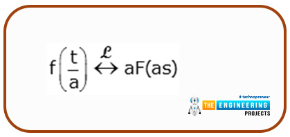
Time scaling
Time scaling is a basic property of signals, and when we talk about the Laplace transform, we get to know that after scaling, the variable a from the denominator is shifted into the multiplication; that is, we get the time signal in the frequency domain.

The Step Function of the Laplace Transform
Here is another thing about the Laplace transform. The step function is defined when we use the function of the following form:
u(t) = ( 0 for t < 0,
1 for t > 0)
This statement shows that for the values between 0 and 1, this statement is also known as the Heaviside function.
Inverse Laplace Transform
As you can guess from the name, the Laplace transform can be inverted, and this procedure is called the inverse transform. Once you transform the function from the time domain to the frequency domain (that's what the Laplace transform does), you can simply invert the whole process by using the inverse Laplace and get the result in the time domain again. This technique is useful in a number of applications of the Laplace transform. It is represented as:
f(t) = L-1{F(s)}
Now coming towards the solution to this transform. While checking the table, you can easily find the inverse transform. However, if the solution or the term is not present in the table, you can find this inverse with the help of the partial fraction expansion method.
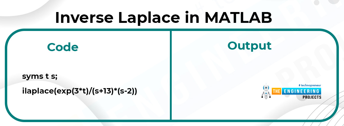
Inverse Laplace in MATLAB
As in the previous case, inverse Laplace is also performed in MATLAB with the help of functions. Here is the simplest example of this function. Suppose we want to perform the inverse transform of the code that we have discussed before.
Code:
syms t s;
ilaplace(exp(3*t)/(s+13)*(s-2))
Output:

All the descriptions are the same as in the previous case, but you can see we used a slightly different function as
ilaplace(x)
Where x is the value of the question that we have fed into this function. Finally, have a look at the code given next in which I just have merged Laplace transform with the inverse Laplace so that you may understand the whole mechanism.
Code:
syms t a s;
f=exp(a*t) %Question
F=laplace(f) %Laplace Transform
G=ilaplace(f) %Inverse Laplace Transform
Output:

Here, a new thing is introduced in our program that may be new to you. We used the comments and these can be added to any program of MATLAB same as the other programming languages.
What are comments in a programming language?
Comments in the programming languages are ignored by the compiler at compile time. In other words, we can not add any extra words in programming languages because the compiler does not understand them and we risk an error. So, if a person wants to add details about the steps or wants to add any notes, he or she uses the comments. The compiler then ignores these lines, and in this way, we do not get any errors. Usually, comments are shown in a different color than the code lines (green in MATLAB). To add comments in the program, we simply put a percentage sign % before the notes.
Partial Fraction Expansion and Inverse Laplace Transform
As we have all learned in our matriculation, the partial fraction is the method in which the difficult denominator is solved by converting it into different partial fractions. In this way, it becomes easy to find the values of variables, and after that, the result is recollected into the desired form.
There are different cases in the partial fraction of the Laplace transform and some of them are given next:
Direct real roots
Repeated real roots
Complex roots
Order of numerator and denominator are equal.
Exponential in the numerator
Now, you must be thinking about how inverse Laplace can be used as a partial fraction. Let's have a simple example in which you will learn to solve this case.
Consider the following question:
F(s)= s^2 +3/s^2(s+2)
You have to follow the steps given next:
Write the right-hand side part of this equation on the left side of the equal sign and mark it as X.
At the right side of the equal sign, you have to split the denominator. Here, you can see that there will be three fractions when we split the denominator. These are:
s
s^2
s+2
The numerator is ignored at this point, and you have to put A, B, and C on each numerator of the partial fraction.
Now, simply multiply s with the whole equation and solve them one after the other.
Cancel the values as much as possible.
Solve the equation.
Repeat the previous four steps by placing the 2nd and 3rd denominator values.
You will find the values of A, B, and C.
Put the values in equation X and this is the required answer.
This explanation is just for revision, otherwise, we all know the implementation of a partial fraction.
Partial Fraction and Laplace Transform in MATLAB
As you were expecting, MATLAB has the implementation of fractions in just a second. You do not have to do long conversions. Simply put the code in MATLAB and you will get accurate and easy answers in just a second.
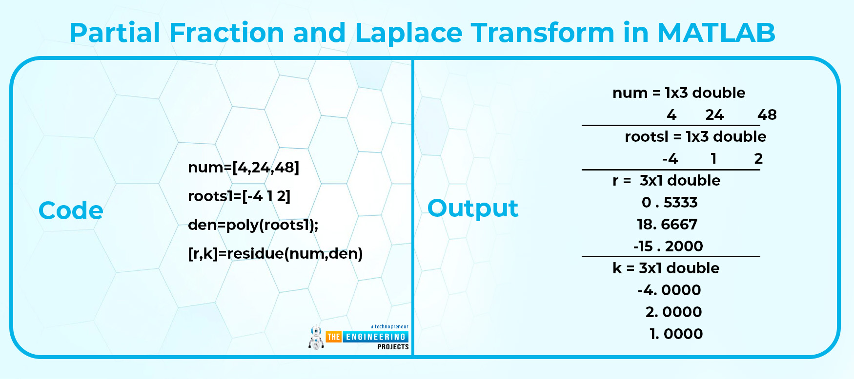
Suppose we have the question:
F(s)=(4s+24s^22+48^3)/(s+4)(s+1)(s+2)
Then you will use the following code.
Code:
num=[4,24,48]
roots1=[-4 1 2]
den=poly(roots1);
[r,k]=residue(num,den)
Output:

Here, you can see that we have used a different type of code that till now we have not discussed. So have a look at the description given next:
The term "num" describes the values in the numerator.
The den represents the entries of the denominator.
We used the poly(x) function in which x represents the value that has to be converted into polynomial form.
Here in the place of x, we inserted the values that, before calling it, we stored in the user-defined variable roots1. It was named by us, but you can call it by any other name.
[r,k] = residue (num, den) is the pre-defined function of MATLAB in which we find the values of the variables that we have shown by storing them in num and den.
Always keep in mind that the values that we have stored in the den are the values when we put the s-x=0, the sign of each value is reversed. Moreover, never change the sequence of the numerator or denominator in the pre-defined function otherwise, you will get different results.
Applications of the Laplace Transform
Have a quick review of the Laplace transform here:
Data mining
In data mining, there is a great role for databases and records of previous values. The laplace transform plays an important role there and helps to keep the record in a great way.
Signal processing
All the conversation about the Laplace transform was based upon the application of this transform in signal processing. It is used in the filtering of signals, processing of signals, and changing the domain of the signals.
Control system
This transform is used to convert the governing complex equations into simple differential equations.
Probability
Not only in probability, but it is also used in the moment and variance as well. It is a necessary topic in most mathematical courses.
Integrated system
In computer ICs, the Laplace transform is used to measure and predict the current and other parameters in a great way. Therefore, it is used in the designing of ICs and delicate circuits in a great way.
Today we have seen some interesting facts about the Laplace transform and read thoroughly about the properties and types of Laplace transforms. We used MATLAB for examples, and we also found the working of this transform in detail. In the end, we have a glance at some basic and simple applications of Laplace transforms.


