
Types of Convolution in MATLAB


Hey pupils, Welcome to another lecture of this series on signals and systems, and this is the time to learn an interesting topic in which you are going to learn about the convolution of the signals. In the previous sessions, we have learned basic operations on the signals, and this time, you are going to know the convolution of the signals and different criteria that are related to this topic. Have a quick view of the concepts that will be clarified in this lecture:
What is convolution?
What are some basic types of convolution?
How can you define the properties of linear convolution?
How can you implement convolution in MATLAB using function and without function?
What is the difference between linear and circular convolution?
What is the convolution of signals?
Convolution is a mathematical operation and it is widely used in signals and systems by using a minimum of two signals at a time. The basic definition of convolution is:
The term "convolution" refers to a mathematical process combining two signals by overlapping them to produce a third signal.
It is important because it establishes a connection between the system's input signal and the impulse response of the system, which determines the system's output, which is utilized to provide a relationship within the LTI system.
Before going into details of the convolution, you must have the idea of shifting and scaling that we have discussed before in this series. Let’s recall them.
"Time shifting" refers to moving a signal forward or backward in time. The time variable in the function is multiplied by the shift or subtracted from it to do this."
Hence, convolution is an integral function that is used to measure the amount of overlap of one function when it is shifted over the other function.
The formula of Convolution
If the definition of convolution is clear to you, then you can easily understand the formula for it.
We all know that there are two types of signals and, therefore, there is a different representation of the formula of convolution in each type.
Convolution of a continuous-time system:
Where,
y(t) = convoluted result
x(t)= 1st function
h(t)= 2nd function
Convolution for a discrete-time system:
Similar to the 1st case,
y(n) = convoluted result
x(n)= 1st function
h(n)= 2nd function
The steric sign here represents convolution, and it is the most important part of this formula. Do not be confused with the symbols of t and k in continuous and discrete signals, respectively. These are the dummy variables of the result so that the input and output representation must not change.
We are not going into details of the derivation but for the clear concepts, let’s solve the example to have practice.
Types of Convolution
Basically, there are two types of convolution that are used in signal and system. These are
Linear convolution
Circular convolution
A brief description of each of them is given next:
Linear Convolution
This is the basic type of convolution and is defined as:
“The calculation of the output of any Linear-Time Invariant (LTI) system, given that system's input and impulse response, is done with the help of a mathematical procedure known as linear convolution.”
Till now, the properties and procedures that we have discussed were related to linear convolutions. One thing that must be kept in mind is, that the arrow on the values of x(t) and h(t) indicates the zero position of the function. If this arrow is not specified, then by default, the first value is the zero value.
Procedure for Linear Convolution of Signals
You will find different formulas to have the convolution of signals, but here, we are providing you with the basic and easiest way to solve the convolution without any confusion. Just follow these simple steps to get the convolution.
Replace T with t
Time reversal in h(t)= h(-t)
Time shifting in h(t)= h(t-t)
Multiplication of h(t-t) with x(t)
Integration of the result by taking the limits from minus infinity to infinity
Keep in mind, in all the steps, the value of x(t) remains the same and just t is replaced by t i.e, time reversal and time shifting do not apply to x(t) while you are using the convolution.
Circular Convolution
The other type that I found more interesting in the convolution of signals is circular convolution. This type can be performed using two different methods, and by observing the procedure of each type, you will understand why this type is called “Circular” convolution. The total number of samples in circular convolution is equal to the maximum number of values in x(t) or h(t). Have a look at both of these:
Concentric circular convolution
Matrix circular convolution
We are going to discuss both of them in the next section.
Concentric circular convolution
Here, you need a circle for each signal or function. In this way, you will have two circles. Follow the steps from the beginning as mentioned below:
Draw a big circle on the page and write the values of x(t) on it at regular intervals.
Draw a relatively small circle inside the first one and write all the values of h(t) on it at the same regular intervals.
Multiply the respective values of both the circles and at the end, add them all. You will get a number.
Now, draw the same circle once again but this time, you have to move the internal circle (the one with h(t) values) one place anti-clockwise and then repeat the above procedure till you get all the values.
Matrix circular convolution
The matrix multiplication, as the name implies, consists of two matrices having the values of x(t) and h(t) respectively. The simple steps involved in this method are:
One of the given sequences is repeated, one sample at a time, to produce an N X N matrix.
The other sequence is shown as a column matrix.
The outcome of circular convolution is obtained by multiplying two matrices.
Convolution Procedure in MATLAB
Here comes the action. You have seen that there were different ways of convolution, and honestly speaking, these procedures are long yet easy. MATLAB has built-in functions for convolution so that you may get the answer to long and time-taking calculations in just a bit. You just have to simply input the values, and tell MATLAB that you want to do the convolution of this signal. Let’s implement all the discussions in MATLAB and get the instant and authentic result of convolution there.
Step for Linear Convolution in MATLAB
Fire up your MATLAB software.
Go to live editor or command window to write the code.
Click the “Run” button.
Save program.
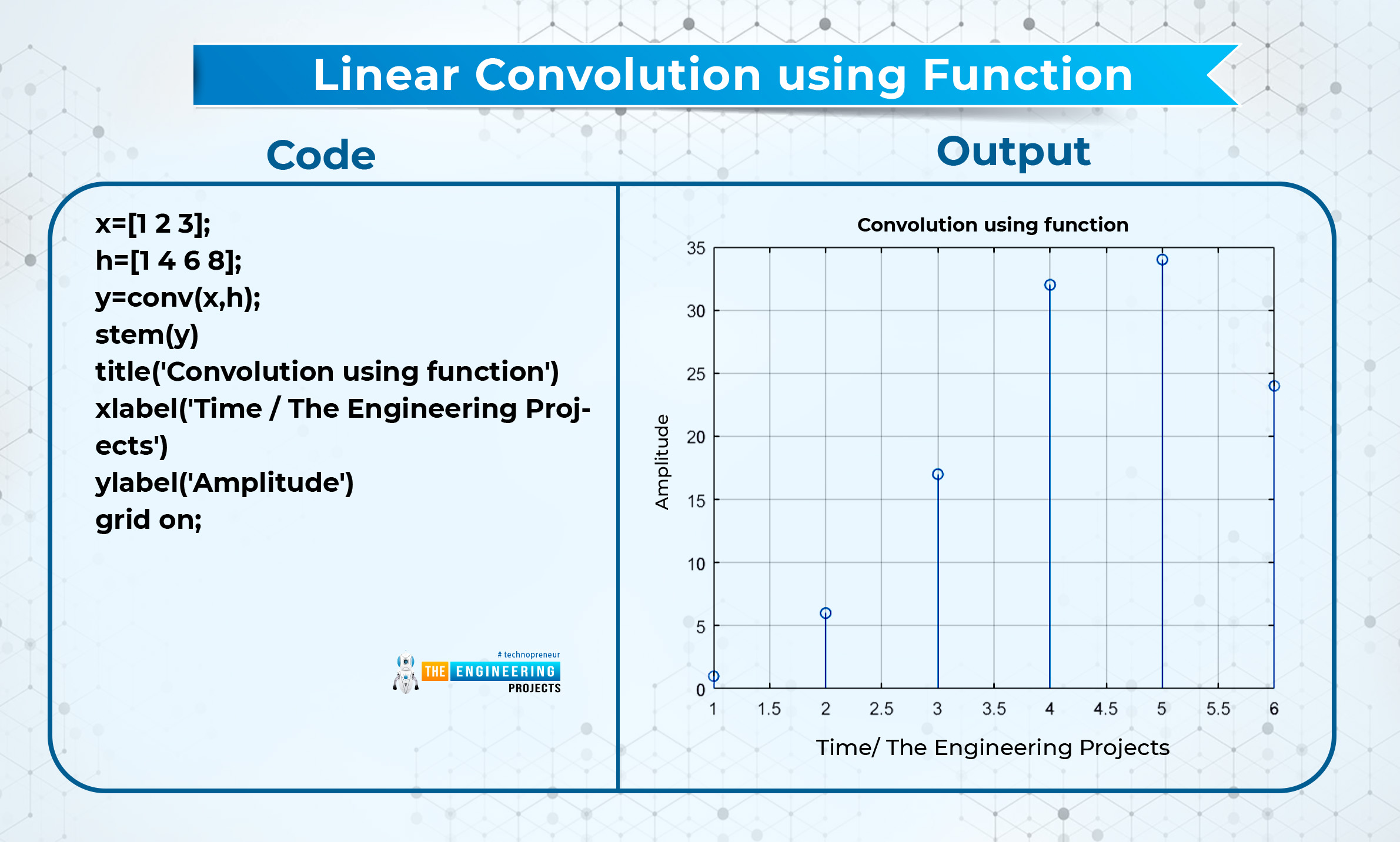
Linear Convolution using Function
There is a built-in function in MATLAB that is super easy to use, and you do not have to go deep into the procedure. You just have to simply provide the input signals and use the convolution function. If x and h are two signals that have the values, then using this function, you can easily convolute them as
conv(x,h)
At the end, you just have to simply put this value in the y variable so that you can plot or stem it easily. Here is the code and output.
Code | Output |
x=[1 2 3]; h=[1 4 6 8]; y=conv(x,h); stem(y) title('Convolution using function') xlabel('Time / The Engineering Projects') ylabel('Amplitude') grid on; |
|
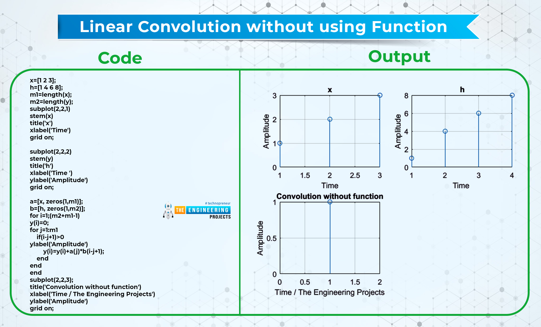
Linear Convolution without using Function
It may come into your exam that you are required to perform the linear convolution but without the help of function. Usually, it happens when the instructor wants to check the knowledge and concept of the student. So here is a simple program for this.
Code | Output |
x=[1 2 3]; h=[1 4 6 8]; m1=length(x); m2=length(y); subplot(2,2,1) stem(x) title('x') xlabel('Time') grid on; subplot(2,2,2) stem(y) title('h') xlabel('Time ') ylabel('Amplitude') grid on; a=[x, zeros(1,m1)]; b=[h, zeros(1,m2)]; for i=1;(m2+m1-1) y(i)=0; for j=1:m1 if(i-j+1)>0 ylabel('Amplitude') y(i)=y(i)+a(j)*b(i-j+1); end end end subplot(2,2,3); title('Convolution without function') xlabel('Time / The Engineering Projects') ylabel('Amplitude') grid on; |
|
Circular Convolution in MATLAB
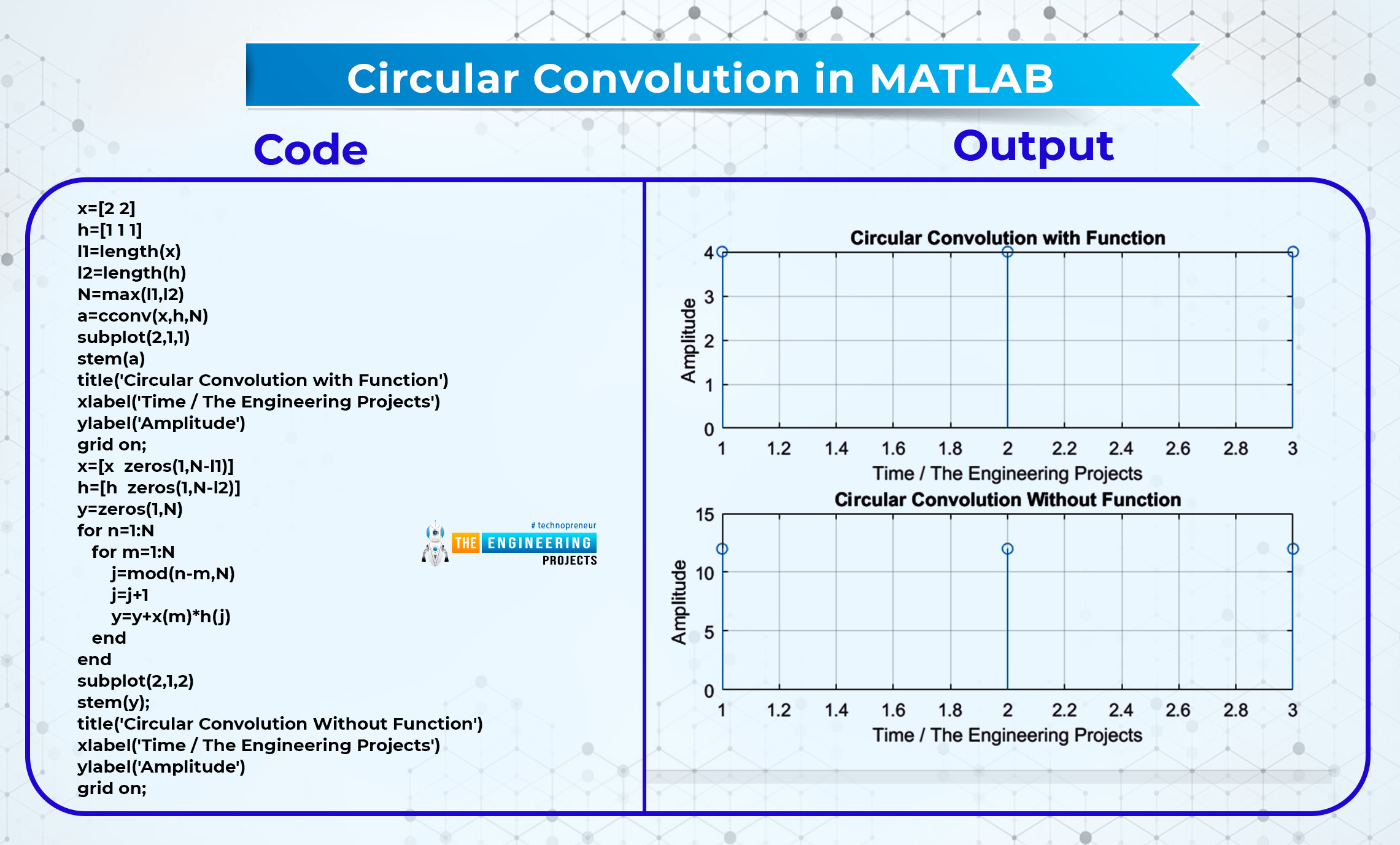
Circular convolution can also be done with the help of function and without it as well. Of course, it is easier to use the function, but in some cases, if you do not want to use the function, it is also possible to do it without the help of the function. The difference between the formulas is, that the circular convolution involves the third parameter as well. This value is obtained when the total number of values of signals is compared and we get the maximum value. For a practice point of view and to clear up the concepts about the topic, we are also using it without any function.
Code | Output |
x=[2 2] h=[1 1 1] l1=length(x) l2=length(h) N=max(l1,l2) a=cconv(x,h,N) subplot(2,1,1) stem(a) title('Circular Convolution with Function') xlabel('Time / The Engineering Projects') ylabel('Amplitude') grid on; x=[x zeros(1,N-l1)] h=[h zeros(1,N-l2)] y=zeros(1,N) for n=1:N for m=1:N j=mod(n-m,N) j=j+1 y=y+x(m)*h(j) end end subplot(2,1,2) stem(y); title('Circular Convolution Without Function') xlabel('Time / The Engineering Projects') ylabel('Amplitude') grid on; |
|
Length Function
Similar to some other functions, length is also a function of MATLAB that stores the output of the number of values that are fed into this function. Let's suppose if the number of elements on the x-axis in a signal is ten and we feed the signal into this function, then it will provide us with the length of 10. It may seem simple, but in complex signals where a hundred or thousand values in a signal are used, this function proves very helpful.
The Max function in MATLAB
Have you observed a function “Max” in the code? It is a built-in function of MATLAB that compares the entries and provides you with the entry (signal in our case) with the maximum number of values. Usually, the answer is then fed into a variable so that we can use the result of this max function anywhere without any difficulty.
For your information, we must share that there is another function named "min", and as you can guess, it does the opposite work. Two or more values are given to this function as well and it compares and then provides the minimum value between these two. It may seem a small task but if used correctly, these functions give us control of many useful things by using them in our program.
Difference Between Linear Convolution and Circular Convolution
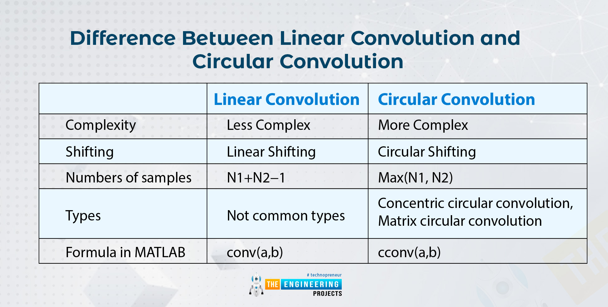
Linear Convolution | Circular Convolution | |
Complexity | Less Complex | More Complex |
Shifting | Linear Shifting | Circular Shifting |
Numbers of samples | N1+N2-1 | Max(N1, N2) |
Types | Not common types | Concentric circular convolution, Matrix circular convolution |
Formula in MATLAB | conv(a,b) | cconv(a,b) |
Conclusion
Convolution is an important topic in signals and systems as it is used to overlap the two signals on each other in such a way that a third signal is obtained that is different from the first two. We have read some important properties of linear convolution and also seen the performance of each type with and without the function in MATLAB. The purpose of providing the program of convolution without function is to clearly describe the concept and the method of convolution. If you have any type of question regarding the topic, you can contact us.


 1 user


 Continue Wishlist


 Getting Started Guide
 Help Center
 Contact us
 Doist Blog
 Privacy
 Security
 Terms of Service
 What's new: Channel Descriptions


 MATLAB
 syedzainnasir
 0 Comments


 2.3k
2.3k
 953
953
 921
921
 2.1K
2.1K


 Convolution and its Types
convolution in matlab
convolution types
convolution basics
 Friday, September 2, 2022